Over/under estimation factor for ‘most estimates’
When asked to estimate the time taken to perform a software development related task, people regularly over or under estimate. What range of over/under estimation falls within the bounds of the term ‘most estimates’, i.e., the upper/lower bounds of the ratio  (an overestimate occurs when
  , an underestimate when
  )?
)?
On Twitter, I have been citing a factor of two for over/under time estimates. This factor of two involves some assumptions and a personal interpretation.
The following analysis is based on the two major software task effort estimation datasets: SiP and CESAW. The tasks in both datasets are for internal projects (i.e., no tendering against competitors), and require at most a few hours work.
The following analysis is based on the SiP data.
Of the 8,252 unique tasks in the SiP data, 30% are underestimates, 37% exact, and 33% overestimates.
How do we go about calculating bounds for the over/under factor of most estimates (a previous post discussed calculating an accuracy metric over all estimates)?
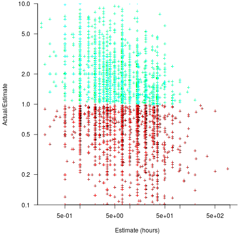
A simplistic approach is to average over each of the overestimated and underestimated tasks. The plot below shows hours estimated against the ratio actual/estimated, for each task (code+data):

Averaging the over/under estimated tasks separately (using the geometric mean) gives 0.47 and 1.9 respectively, i.e., tasks are over/under estimated by a factor of two.
This approach fails to take into account the number of estimates that are over/under/equal, i.e., it ignores likelihood information.
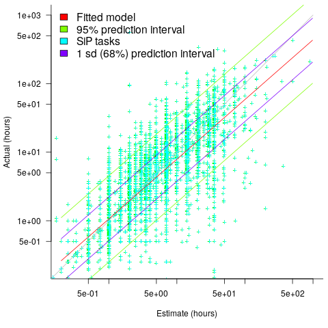
A regression model takes into account the distribution of values, and we could adopt the fitted model’s prediction interval as the over/under confidence intervals. The prediction interval is the interval within which other observations are expected to fall, with some probability (R’s predict function uses one standard deviation).
The plot below shows a fitted regression model and prediction intervals at one standard deviation (68.3%) and two standard deviations (95%); the faint grey line shows Estimate == Actual (code+data):

The fitted model tilts down from the upward direction of the Estimate == Actual line, consequently the over/under estimation factor depends on the size of the estimate. The table below lists the over/under estimation factor for low/high estimates at one & two standard deviations (68.3 and 95% probability).
People like simple answers (i.e., single values) and the mean value is a commonly used technique of summarising many values. The task estimate values are unevenly distributed and weighting the mean by the distribution of estimated values is more representative than, say, an evenly distributed set of estimates. The 5th and 6th columns in the table below list the weighted means at one/two standard deviations (the CESAW columns are the values for all projects in the CESAW data).
          1 sd           2 sd        Weighted mean       CESAW
       Low    High   Low    High     1 sd    2 sd     1 sd   2 sd
Over   0.56   0.24   0.27   0.11     0.46    0.25     0.29   0.1
Under 2.4 1.0 4.9 2.0 2.00 4.1 2.4 6.5 |
The weighted means for over/under estimates are close to a factor of two of the actual (divide/multiply) within one standard deviation (68.3%), and a factor of four within two standard deviations (95%).
Why choose to give the one standard deviation factor, rather than the two? People talk of “most estimates”, but what percentage range does ‘most’ map to? I have tended to think of ‘most’ as more than two-thirds, e.g., at least one standard deviation (a recent study suggests that ‘most’ usage peaks at 80-85%), and I think of two standard deviations as ‘nearly all’ (i.e., 95%; there are probably people who call this ‘most’).
Perhaps a between two and four is a more appropriate answer (particularly since the bounds are wider for the CESAW data). Suggestions welcome.
Recent Comments