Archive
R needs some bureaucracy
Writing a program in R is almost bureaucracy free: variables don’t need to be declared, the language does a reasonable job of guessing the type a value might need to be automatically be converted to, there is no need to create a function having a special name that gets called at program startup, the commonly used library functions are ready and waiting to be called and so on.
Not having a bureaucracy is all well and good when programs are small or short lived. Large programs need a bureaucracy to provide compartmentalization (most changes to X need to be prevented from having an impact outside of X, doing this without appropriate language support eventually burns out anybody juggling it all in their head) and long lived programs need a bureaucracy to provide version control (because R and its third-party libraries change over time).
Automatically installing a package from CRAN always fetches the latest version. This is all well and good during initial program development. But will the code still work in six months time? Perhaps the author of one of the packages used in the program submits a new version of that package to CRAN and this new version behaves slightly differently, breaking the previously working program. Once the problem is located the developer has either to update their code or manually install the older version of the package. Life would be easier if it was possible to specify the required package version number in the call to the library function.
Discovering that my code depends on a particular version of a CRAN package is an irritation. Discovering that two packages I use each have a dependency on different versions of the same package is a nightmare. Having to square this circle is known in the Microsoft Windows world as DLL hell.
There is a new paper out proposing a system of dependency versioning for package management. The author proposes adding a version parameter to the library function, plus lots of other potentially useful functionality.
Apart from changing the behavior of functions a program calls, what else can a package author do to break developer code? They can create new functions and variables. The following is some code that worked last week:
library("foo") # The function get_question is in this package library("bar") # The function give_answer_42 is in this package (the_question=get_question()) give_answer_42(the_question) |
between last week and today the author of package foo (or perhaps the author of one of the packages that foo has a dependency on) has added support for the function solve_problem_42 and it is this function that will now get called by this code (unless the ordering of the calls to library are switched). What developers need to be able to write is:
library("foo", import=c("the_question")) # The function get_question is in this package library("bar", import=c("give_answer_42")) # The function give_answer_42 is in this package (the_question=get_question()) give_answer_42(the_question) |
to stop this happening.
The import parameter enables developers to introduce some compartmentalization into my programs. Yes, R does have namespace management for packages, and I’m pleased to see that its use will be mandatory in R version 3.0.0, but this does not protect programs from functions the package author intends to export.
I’m not sure whether this import suggestion will connect with R users (who look very laissez faire to me), but I get very twitchy watching a call to library go off and install lots of other stuff and generate warnings about this and that being masked.
Does native R usage exist?
Note to R users: Users of other languages enjoy spending lots of time discussing the minutiae of the language they use, something R users don’t appear to do; perhaps you spend your minutiae time on statistics which I don’t yet know well enough to spot when it occurs). There follows a minutiae post that may appear to be navel-gazing to you (interesting problem at the end though).
In various posts written about learning R I have said “I am trying to write R like a native”, which begs the question what does R written by a native look like? Assuming for a moment that ‘native R’ exists (I give some reasons why it might not below) how…
To help recognise native R it helps to start out by asking what it is not. Let’s start with an everyday analogy; if I listen to a French/German/American person speaking English I can usually tell what country they are from, they have patterns of usage that we in merry England very rarely, if ever, use; the same is true for programming languages. Back in the day when I spent several hours a day programming in various languages I could often tell when somebody showing me some Pascal code had previously spent many years writing Fortran or that although they were now using Fortran they had previously used Algol 60 for many years.
If expert developers can read R source and with high accuracy predict the language that its author previously spent many years using, then the source is not native R.
Having ruled out any code that is obviously (to a suitably knowledgeable person) not native R, is everything that is left native R? No, native language users share common characteristics; native speakers recognize these characteristics and feel at home. I’m not saying these characteristics are good, bad or indifferent any more than my southern English accent is better/worse than northern English or American accents; it is just the way people around here speak.
Having specified what I think is native R (I would apply the same rules to any language) it is time to ask whether it actually exists.
I’m sure there are people out there whose first language was R and who have spent a lot more time using R over, say, five years rather than any other language. Such people are unlikely to have picked up any noticeable coding accents from other languages and so can be treated as native.
Now we come to the common characteristics requirement, this is where I think an existence problem may exist.
How does one learn to use a language fluently? Taking non-R languages I am familiar with the essential ingredients seem to be:
- spending lots of time using the language, say a couple of hours a day for a few years
- talking to other, heavy, users of the language on a daily basis (often writing snippets of code when discussing problems they are working on),
- reading books and articles covering language usage.
I am not saying that these activities create good programmers, just that they result in language usage characteristics that are common across a large percentage of the population. Talking and reading provides the opportunity to learn specific techniques and writing lots of code provides the opportunity to make use these techniques second nature.
Are these activities possible for R?
- I would guess that most R programs are short, say under 150 lines. This is at least an order of magnitude shorter (if not two or three orders of magnitude) than program written in Java/C++/C/Fortran/etc. I know there are R users out there who have been spending a couple of hours a day using R over several years, but are they thinking about R coding or think about the statistics and what the data analysis really means. I suspect they are spending most of this R-usage thinking time on the statistics and data analysis,
- I can easily imagine groups of people using R and individuals having the opportunity to interact with other R users (do they talk about R and write snippets of code to describe their problem? I don’t work in an R work environment, so I don’t know the answer),
- Where are the R books and articles on language usage? They don’t exist, not in the sense of Sutter’s “Effective C++: 55 Specific Ways to Improve Your Programs and Designs” (there must be a several dozen of this kind of book for C++) Bloch’s “Java Puzzlers: Traps, Pitfalls, and Corner Cases” (probably only a handful for Java) and Koenig’s “C: Traps and Pitfalls” (again a couple of dozen for C). In places Crawley’s “The R Book” has the feel of this kind of book, but Matloff’s “The Art of R Programming” is really an introduction to R for people who already know another language (no discussion of art of R as such). R users write about statistics and data analysis, with the language being a useful tool.
I suspect that many people are actually writing R for short amounts of time to solve data analysis problems they spend a lot of time thinking about; they don’t discuss R the language much (so little opportunity to learn about the techniques that other people use) and they don’t write much code (so little opportunity to try out many new techniques).
Yes, there may be a few people who do spend a couple of hours a day thinking about R the language and also get to write lots of code, these people are more like high priests than your average user.
For the last two years I have been following a no for-loops policy in an attempt to make myself write R how the natives write it. I am beginning to suspect that this view of native R is really just me imposing beliefs from usage of other language that support whole vector/array operations, e.g., APL.
I encountered the following coding problem yesterday. Do you think the non-loop version should be how it is done in R or is the loop version more ‘natural’?
Given a vector of ordered items the problem is to count the length of each subsequence of identical items,
a,a,a,b,b,a,c,c,c,c,b,c,c |
output
a 3 b 2 a 1 c 4 b 1 c 2 |
Non-looping version (looping version is easy to figure out):
subseq_len=function(feature) { r_shift=c(feature[1], feature) l_shift=c(feature, ",,,") # pad with something that will not match # Where are the boundaries between subsequences? boundary=(l_shift != r_shift) sum_matches=cumsum(!boundary) # Difference of cumulative sum at boundaries, whose value will # be off by 1 and we need to handle 'virtual' start of list at 1. t=sum_matches[boundary] seq_len=1+c(t, 0)-c(1, t) # Remove spurious value return(cbind(feature[boundary[-1]], seq_len[-length(seq_len)])) } subseq_len(c("a", "a", "b", "b", "e", "c", "c", "c", "a", "c", "c")) |
My R naming nemesis
When learning a new language I try to make an effort to write it like a native developer. R has one language feature that has been severely testing my desire to write like a native and this afternoon I realized that most of the people reading my code will also experience the same jarring sensation on encountering this construct, so I am not going to use it any more.
What is this language feature that induces a Stroop effect in my mind? It is the use of the period character as part of an identifier’s name (e.g., foo.bar). In almost all of the hundreds of thousands of lines of code I have read over the years this character is used as an operator, it selects a member/field of a struct/record. I’m sure that if I tried long enough and hard enough I could get used to using this character being part of an identifier; after a year or so writing Cobol I got used to the arithmetic minus character being permitted within identifiers (e.g., foo-bar), but that was 20 years ago and my neurons will probably take much longer to adapt this time around.
Most of the R I am writing will be distributed with my book Empirical software engineering with R and I think readers will experience the same jarring sensation I do (apart from those who have not yet been exposed to large amounts of non-R code). I have convinced myself that this is a good enough reason to give up trying to figure out how to use . in identifier name (I have been concocting all sorts of rules involving . being used to separate the primary part of the name and _ the secondary parts, e.g., total.red_light [yes, I should get out more often]; the underscore vs. camel case debate still erupts every now and again, let’s avoid creating more debate by introducing more choice).
Those R functions that include a . in their name will stand out from the crowd, [arm waving on] perhaps this will help differentiate them as ‘statistics stuff'[arm waving off]. There is always plan B if my unilateral naming decision looks too unilateral, a global renaming script.
Perhaps the use of periods in identifiers can be used as a test for being a native R developer. A simple timing test involving a sequence of characters appears on a screen with the developer having to respond as quickly as possible on the number of identifiers being displayed; I’m sure I would be much slower to give a ‘1’ response to total.count than to total_count, displaying total count and total.count on twp separate lines and asking me to quickly specify which line contained the most identifiers would turn me into a nervous wreck. Responses from a dozen or so different sequences ought to be enough be able to distinguish Jonny foreigner from the natives.
I don’t have a problem with $, which R uses as the column/list item selection operator, a character permitted by some compilers for commonly used languages as part of an identifier. This is because I have not read lots of code containing this identifier naming usage.
For my previous book I did a survey of the linguistic and cognitive psychology issues involved in identifier naming. This did a good job of debunking existing ideas about what constitutes good naming practices, but did not come up with any concrete recommendations to replace them (nature abhors a vacuum and the existing pop psychology naming ideas remained).
These days people write PhDs on identifier naming issues (method names, (not yet completed) correlation with quality and code comprehension to name a few); there is even a subfield within this field, how best to split an identifier into its component parts (e.g., refPtr is probably an abbreviation of reference pointer).
Distribution of uptimes for high-performance computing systems
Computers break down every now and again and this is a serious problem when an application needs runs on thousands of individual computers (nodes) plugged together; lots more hardware creates lots more opportunity for a failure that renders any subsequent calculations by working nodes possible wrong. The solution is checkpointing; saving the state of each node every now and again, and rolling back to that point when a failure occurs. Picking the optimal interval between checkpoints requires knowledge the distribution of node uptimes, what is it?
Short answer: Node uptimes have a negative binomial distribution, or at least five systems at the Los Alamos National Laboratory do.
The longer answer is below as another draft section from my book Empirical software engineering with R. As always comments and pointers to more data welcome. R code and data here.
Distribution of uptimes for high-performance computing systems
Today’s high-performance computing systems are created by connecting together lots of cpus. There is a hierarchy to the connection in that many cpus may populate a single board, several boards may be fitted into a rack unit, several rack units into a cabinet, lots of cabinets lined up in a row within a room and more than one room in a facility. A common operating unit is the node, effectively a computer on which an operating system is running (the actual hardware involved may be a single or multi processor cpu). A high-performance system is built from thousands of nodes and an application program may run on compute nodes from more than one facility.
With so many components, failures occur on a regular basis and long running applications need to recover from such failures if they are to stand a reasonable chance of ever completing.
Applications running on the systems installed at the Los Alamos National Laboratory create checkpoints at regular intervals, writing data needed to do a full restore to storage. When a failure occurs an application is restarted from its most recent checkpoint, one node failure causes all nodes to be rolled back to their most recent checkpoint (all nodes create their checkpoints at the same time).
A tradeoff has to be made between frequently creating checkpoints, which takes resources away from completing execution of the application but reduces the amount of lost calculation, and infrequent checkpoints, which diverts less resources but incurs greater losses when a fault occurs. Calculating the optimum checkpoint interval requires knowing the distribution of node uptimes and the following analysis attempts to find this distribution.
Data
The data comes from 23 different systems installed at the Los Alamos National Laboratory (LANL) between 1996 and 2005. The total failure count for most of the systems is of the order of a few hundred; there are five systems (systems 2, 16, 18, 19 and 20) that each have several thousand failures and these are the ones analysed here.
The data consists of failure records for every node in a system. A failure record includes information such as system id, node number, failure time, restored to service time, various hardware characteristics and possible root causes for the failure. Schroeder and Gibson <book Schroeder_06> performed the first analysis of the dataset and provide more background details.
Is the data believable?
Failure records are created by operations staff when they are notified by the automated monitoring system that a failure has been detected. Given that several people are involved in the process <book LANL_data_06> it seems unlikely that failures will go unreported.
Some of the failure reports have start times before the given node was returned into service from the previous failure; across the five systems this varied between 0.4% and 2.5%. It is possible that these overlapping failures are caused by an incorrectly attempt to fix the first failure, or perhaps they are data entry errors. This error rate is comparable with human error rates for low stress/non-critical work
The failure reports do not include any information about the application software running on the node when it failed; the majority of the programs executed are large-scale scientific simulations, such as simulations of nuclear stockpile stability. Thus it is not possible to accurately calculate the node MTBF for an executing application. LANL say <book LANL_data_06> that the applications “… perform long periods (often months) of CPU computation, interrupted every few hours by a few minutes of I/O for check-pointing.”
Predictions made in advance
The purpose of this analysis is to find the distribution that best fits the node uptime data, i.e., the time interval between failures of the same node.
Your author is not aware of any empirically based theory that predicts the uptime of high performance computing systems. The Poisson and exponential distributions are both frequently encountered in the analysis of hardware failures and it is always comforting to fit in with existing expectations.
Applicable techniques
A [Cullen and Frey test] matches a dataset’s skew and kurtosis against known distributions (in the case of the descdist function in the fitdistrplus package this is a handful of commonly encountered distributions); the fitdist function in the same package can be used to fit the data to a specified distribution.
Results
The table below lists some basic properties of each of the systems analysed. The large difference in mean/median uptimes between some systems is caused by very fat tails in the uptime distribution of some systems, see [LANL-node-uptime-binned].
| System | Nodes | Failures | Mean | Median |
|---|---|---|---|---|
|
2
|
49
|
6997
|
133
|
377
|
|
16
|
16
|
2595
|
89
|
229
|
|
18
|
823
|
3014
|
2336
|
4147
|
|
19
|
738
|
2344
|
2376
|
4069
|
|
20
|
323
|
2063
|
653
|
2544
|
If there are any significant changes in failure rate over time or across different nodes in a given system it could have a significant impact on the distribution of uptime intervals. So we first check to large differences in failure rates.
Do systems experience any significant changes in failure rate over time?
The plot below shows the total number of failures, binned using 30-day periods, for the five systems. Two patterns that stand out are system 20 which experienced many failures during the first few months and then settled down, and system 2’s sudden spike in failures around month 23 before settling down again. This analysis is intended to be broad brush and does not get involved with details of specific systems, but these changes in failure frequency suggest that the exact form of any fitted distribution may change over time in turn potentially leading to a change of checkpoint interval.
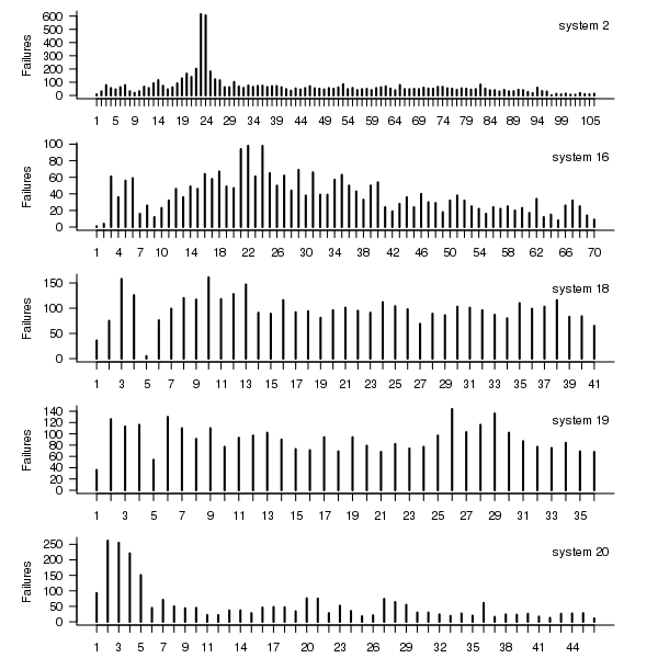
Figure 1. Total number of failures per 30-day interval for each LANL system.
Do some nodes failure more often than others?
The plot below shows the total number of failures for each node in the given system. Node 0 has many more failures than the other nodes (for node 0 of system 2 most of the failure data appears to be missing, so node 1 has the most failures). The distribution suggested by the analysis below is not changed if Node 0 is removed from the dataset.
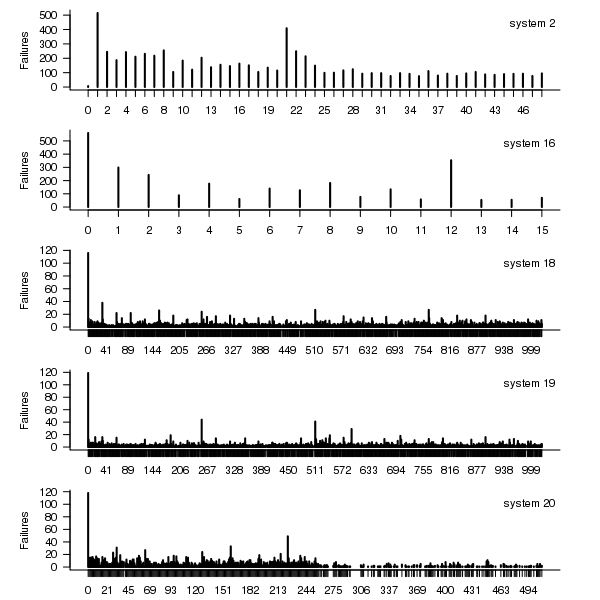
Figure 2. Total number of failures for each node in the given LANL system.
Fitting node uptimes
When plotted in units of 1 hour there is a lot of variability and so uptimes are binned into 10 hour units to help smooth the data. The number of uptimes in each 10-hour bin forms a discrete distribution and a [Cullen and Frey test] suggests that the negative binomial distribution might provide the best fit to the data; the Scroeder and Gibson analysis did not try the negative binomial distribution and of those they tried found the Weilbull distribution gave the best fit; the R functions were not able to fit this distribution to the data.
The plot below shows the 10-hour binned data fitted to a negative binomial distribution for systems 2 and 18. Visually the negative binomial distribution provides the better fit and the Akaiki Information Criterion values confirm this (see code for details and for the results on the other systems, which follow one of the two patterns seen in this plot).
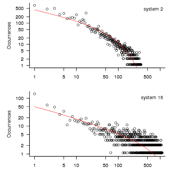
Figure 3. For systems 2 and 18, number of uptime intervals, binned into 10 hour interval, red line is fitted negative binomial distribution.
The negative binomial distribution is also the best fit for the uptime of the systems 16, 19 and 20.
The Poisson distribution often crops up in failure analysis. The quality of fit of a Poisson distribution to this dataset was an order of worse for all systems (as measured by AIC) than the negative binomial distribution.
Discussion
This analysis only compares how well commonly encountered distributions fit the data. The variability present in the datasets for all systems means that the quality of all fitted distributions will be poor and there is no theoretical justification for testing other, non-common, distributions. Given that the analysis is looking for the best fit from a chosen set of distributions no attempt was made to tune the fit (e.g., by forming a zero-truncated distribution).
Of the distributions fitted the negative binomial distribution has the lowest AIC and best fit visually.
As discussed in the section on [properties of distributions] the negative binomial distribution can be generated by a mixture of [Poisson distribution]s whose means have a [Gamma distribution]. Perhaps the many components in a node that can fail have a Poisson distribution and combined together the result is the negative binomial distribution seen in the uptime intervals.
The Weilbull distribution is often encountered with datasets involving some form of time between events but was not seen to be a good fit (for a continuous distribution) by a Cullen and Frey test and could not be fitted by the R functions used.
The characteristics of node uptime for two systems (i.e., 2 and 16) follows what might be thought of as a typical distribution of measurements, with some fattening in the tail, while two systems (i.e., 18 and 19) have very fat tails with indeed and system 20 sits between these two patterns. One system characteristic that matches this pattern is the number of nodes contained within it (with systems 2 and 16 having under 50, 18 and 19 having over 1,000 and 20 having around 500). The significantly difference in the size of the tails is reflected in the mean uptimes for the systems, given in the table above.
Summary of findings
The negative binomial distribution, of the commonly encountered distributions, gives the best fit to node uptime intervals for all systems.
There is over an order of magnitude variation in the mean uptime across some systems.
Break even ratios for development investment decisions
Developers are constantly being told that it is worth making the effort when writing code to make it maintainable (whatever that might be). Looking at this effort as an investment what kind of return has to be achieved to make it worthwhile?
Short answer: The percentage saving during maintenance has to be twice as great as the percentage investment during development to break even, higher ratio to do better.
The longer answer is below as another draft section from my book Empirical software engineering with R book. As always comments and pointers to more data welcome. R code and data here.
Break even ratios for development investment decisions
Upfront investments are often made during software development with the aim of achieving benefits later (e.g., reduced cost or time). Examples of such investments include spending time planning, designing or commenting the code. The following analysis calculates the benefit that must be achieved by an investment for that investment to break even.
While the analysis uses years as the unit of time it is not unit specific and with suitable scaling months, weeks, hours, etc can be used. Also the unit of development is taken to be a complete software system, but could equally well be a subsystem or even a function written by one person.
Let  be the original development cost and
  the yearly maintenance costs, we start by keeping things simple and assume
  is the same for every year of maintenance; the total cost of the system over
  years is:

If we make an investment of  % in reducing future maintenance costs with the expectations of achieving a benefit of
  %, the total cost becomes:

and for the investment to break even the following inequality must hold:

expanding and simplifying we get:

or:

If the inequality is true the ratio  is the primary contributor to the right-hand-side and must be greater than 1.
A significant problem with the above analysis is that it does not take into account a major cost factor; many systems are replaced after a surprisingly short period of time. What relationship does the  ratio need to have when system survival rate is taken into account?
Let  be the percentage of systems that survive each year, total system cost is now:

where 
Summing the power series for the maximum of  years that any system in a company’s software portfolio survives gives:

and the break even inequality becomes:

The development/maintenance ratio is now based on the yearly cost multiplied by a factor that depends on the system survival rate, not the total maintenance cost
If we take  >= 5 and a survival rate of less than 60% the inequality simplifies to very close to:

telling us that if the yearly maintenance cost is equal to the development cost (a situation more akin to continuous development than maintenance and seen in 5% of systems in the IBM dataset below) then savings need to be at least twice as great as the investment for that investment to break even. Taking the mean of the IBM dataset and assuming maintenance costs spread equally over the 5 years, a break even investment requires savings to be six times greater than the investment (for a 60% survival rate).
The plot below gives the minimum required saving/investment ratio that must be achieved for various system survival rates (black 0.9, red 0.8, blue 0.7 and green 0.6) and development/yearly maintenance cost ratios; the line bundles are for system lifetimes of 5.5, 6, 6.5, 7 and 7.5 years (ordered top to bottom)
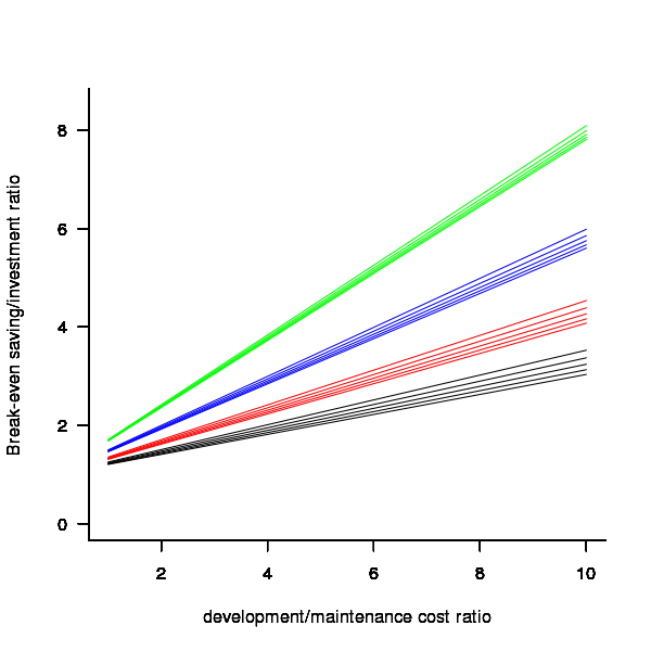
Figure 1. Break even saving/investment ratio for various system survival rates (black 0.9, red 0.8, blue 0.7 and green 0.6) and development/maintenance ratios; system lifetimes are 5.5, 6, 6.5, 7 and 7.5 years (ordered top to bottom)
Development and maintenance costs
Dunn’s PhD thesis <book Dunn_11> lists development and total maintenance costs (for the first five years) of 158 software systems from IBM. The systems varied in size from 34 to 44,070 man hours of development effort and from 21 to 78,121 man hours of maintenance.
The plot below shows the ratio of development to five year maintenance costs for the 158 software systems. The mean value is around one and if we assume equal spending during the maintenance period then  .
.
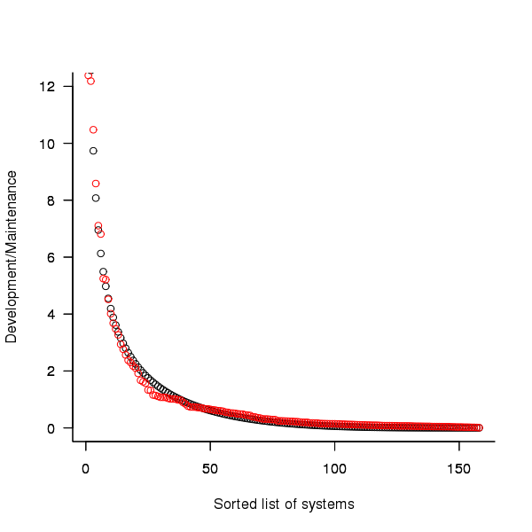
Figure 2. Ratio of development to five year maintenance costs for 158 IBM software systems sorted in size order. Data from Dunn <book Dunn_11>.
The best fitting common distribution for the maintenance/development ratio is the <Beta distribution>, a distribution often encountered in project planning.
Is there a correlation between development man hours and the maintenance/development ratio (e.g., do smaller systems tend to have a lower/higher ratio)? A Spearman rank correlation test between the maintenance/development ratio and development man hours gives:
|
showing very little connection between the two values.
Is the data believable?
While a single company dataset might be thought to be internally consistent in its measurement process, IBM is a very large company and it is possible that the measurement processes used were different.
The maintenance data applies to software systems that have not yet reached the end of their lifespan and is not broken down by year. Any estimate of total or yearly maintenance can only be based on assumptions or lifespan data from other studies.
System lifetime
A study by Tamai and Torimitsu <book Tamai_92> obtained data on the lifespan of 95 software systems. The plot below shows the number of systems surviving for at least a given number of years and a fit of an <Exponential distribution> to the data.
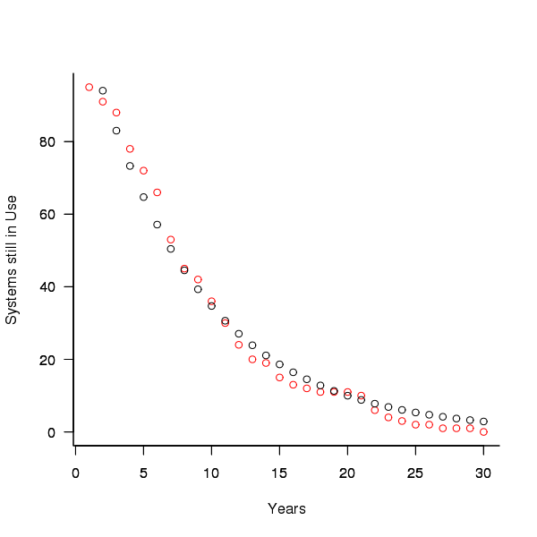
Figure 3. Number of software systems surviving to a given number of years (red) and an exponential fit (black, data from Tamai <book Tamai_92>).
The nls function gives  as the best fit, giving a half-life of 5.4 years (time for the number of systems to reduce by 50%), while rounding to
  gives a half-life of 6.6 years and reducing to
  a half life of 4.6 years.
It is worrying that such a small change to the estimated fit can have such a dramatic impact on estimated half-life, especially given the uncertainty in the applicability of the 20 year old data to today’s environment. However, the saving/investment ratio plot above shows that the final calculated value is not overly sensitive to number of years.
Is the data believable?
The data came from a questionnaire sent to the information systems division of corporations using mainframes in Japan during 1991.
It could be argued that things have stabilised over the last 20 years ago and complete software replacements are rare with most being updated over longer periods, or that growing customer demands is driving more frequent complete system replacement.
It could be argued that large companies have larger budgets than smaller companies and so have the ability to change more quickly, or that larger companies are intrinsically slower to change than smaller companies.
Given the age of the data and the application environment it came from a reasonably wide margin of uncertainty must be assigned to any usage patterns extracted.
Summary
Based on the available data an investment during development must recoup a benefit during maintenance that is at least twice as great in percentage terms to break even:
- systems with a yearly survival rate of less than 90% must have a benefit/investment rate greater than two if they are to break even,
- systems with a development/yearly maintenance rate of greater than 20% must have a benefit/investment rate greater than two if they are to break even.
The availanble software system replacement data is not reliable enough to suggest any more than that the estimated half-life might be between 4 and 8 years.
This analysis only considers systems that have been delivered and started to be used. Projects are cancelled before reaching this stage and including these in the analysis would increase the benefit/investment break even ratio.
Agreement between code readability ratings given by students
I have previously written about how we know nothing about code readability and questioned how the information content of expressions might be calculated. Buse and Weimer ran a very interesting experiment that asked subjects to rate short code snippets for readability (somebody please rerun this experiment using professional software developers).
I’m interested in measuring how well different students subjects agree with each other (I have briefly written about this before).
Short answer: Very little agreement between individual pairs, good agreement between rankings aggregated by year.
The longer answer is below as another draft section from my book Empirical software engineering with R book. As always comments welcome. R code and data here.
Readability
Source code is often said to have an attribute known as
A study by Buse and Weimer <book Buse_08> asked Computer Science students to rate short snippets of Java source code on a scale of 1 to 5. Buse and Weimer then searched for correlations between these ratings and various source code attributes they obtained by measuring the snippets.
Humans hold diverse opinions, have fragmented knowledge and beliefs about many topics and vary in their cognitive abilities. Any study involving human evaluation that uses an open ended problem on which subjects have had little experience is likely to see a wide range of responses.
Readability is a very nebulous term and students are unlikely to have had much experience working with source code. A wide range of responses is to be expected and the analysis performed here aims to check the degree of readability rating agreement between the subjects.
Data
The data made available by Buse and Weimer are the ratings, on a scale of 1 to 5, given by 121 students to 100 snippets of source code. The student subjects were drawn from those taking first, second and third/fourth year Computer Science degree courses and postgraduates at the researchers’ University (17, 65, 31 and 8 subjects respectively).
The postgraduate data was not used in this analysis because of the small number of subjects.
The source of the code snippets is also available but not used in this analysis.
Is the data believable?
The subjects were not given any instructions on how to rate the code snippets for readability. Also we don’t know what outcome they were trying to achieve when rating, e.g., where they rating on the basis of how readable they personally found the snippets to be, or rating on the basis of the answer they would expect to give if they were being tested in an exam.
The subjects were students who are learning about software development and many of them are unlikely to have had any significant development experience outside of the teaching environment. Experience shows that students vary significantly in their ability to read and write source code and a non-trivial percentage do not go on to become software developers.
Because the subjects are at an early stage of learning about code it is to be expected that their opinions about readability will change while they are rating the 100 snippets. The study did not include multiple copies of some snippets, this would have enabled the consistency of individual subject responses to be estimated.
The results of many studies <book Annett_02> has shown that most subject ratings are based on an ordinal scale (i.e., there is no fixed relationship between the difference between a rating of 2 and 3 and a rating of 3 and 4), that some subjects are be overly generous or miserly in their rating and that without strict rating guidelines different subjects apply different criteria when making their judgements (which can result a subject providing a list of ratings that is inconsistent with every other subject).
Readability is one of those terms that developers use without having much idea what they and others are really referring to. The data from this study can at most be regarded as treating readability to be whatever each subject judges it to be.
Predictions made in advance
Is the readability rating given to code snippets consistent between different students on a computer science course?
The hypothesis is that the between student consistency of the readability rating given to code snippets improves as students progress through the years of attending computer science courses.
Applicable techniques
There are a variety of techniques for estimating rater agreement. <Krippendorff’s alpha> can be applied to ordinal ratings given by two or more raters and is used here.
Subjects do not have to give the same rating to share some degree of consistent response. Two subjects may share a similar pattern of increasing/decreasing/stay the same ratings across snippets. The <Spearman rank correlation> coefficient can be used to measure the correlation between the rank (i.e., relative value within sequence) of two sequences.
Results
When creating the snippets the researchers had no method of estimating what rating subjects would give to them and so there is no reason to expect a uniform distribution of rating values or any other kind of distribution of rating values.
The figure below is a boxplot of the rating of the first 50 code snippets rated by second year students and suggests that many subject ratings are within ±1 of each other.
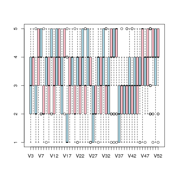
Figure 1. Boxplot of ratings given to snippets 1 to 50 by second year students (colors used to help distinguish boxplots for each snippet).
Between subject rating agreement
The Krippendorff alpha and mean Spearman rank correlation coefficient (the coefficient is calculated for every pair of subjects and the mean value taken) was obtained using the kripp.alpha and meanrho functions from the irr package (a <Jackknife> was used to obtain the following 95% confidence bounds):
Krippendorff's alpha cs1: 0.1225897 0.1483692 cs2: 0.2768906 0.2865904 cs4: 0.3245399 0.3405599 mean Spearman's rho cs1: 0.1844359 0.2167592 cs2: 0.3305273 0.3406769 cs4: 0.3651752 0.3813630 |
Taken as a whole there is a little of agreement. Perhaps there is greater consensus on the readability rating for a subset of the snippets. Recalculating using only using those snippets whose rated readability across all subjects, by year, has a standard deviation less than 1 (around 22, 51 and 62% of snippets respectively) shows some improvement in agreement:
Krippendorff's alpha cs1: 0.2139179 0.2493418 cs2: 0.3706919 0.3826060 cs4: 0.4386240 0.4542783 mean Spearman's rho cs1: 0.3033275 0.3485862 cs2: 0.4312944 0.4443740 cs4: 0.4868830 0.5034737 |
Between years comparison of ratings
The ratings from individual subjects is only available for one of their years at University. Aggregating the answers from all subjects in each year is one method of obtaining readability information that can be used to compare the opinions of students in different years.
How can subject ratings be aggregated to rank the 100 code snippets in order of what a combined group consider to be readability? The relatively large variation in mean value of the snippet ratings across subjects would result in wide confidence bounds for an aggregate based on ratings. Mapping each subject’s rating to a ranking removes the uncertainty caused by differences in mean subject ratings.
With 100 snippets assigned a rating between 1 and 5 by each subject there are going to be a lot of tied rankings. If, say, a subject gave 10 snippets a rating of 5 the procedure used is to assign them all the rank that is the mean of the ranks the 10 of them would have occupied if their ratings had been very slightly different, i.e., (1+2+3+4+5+6+7+8+9+10)/10 = 5.5. This process maps each students readability ratings to readability rankings, the next step is to aggregate these individual rankings.
The R_package[RankAggreg] package contains a variety of functions for aggregating a collection rankings to obtain a group ranking. However, these functions use the relative order of items in a vector to denote rank, and this form of data representations prevents them supporting ranked lists containing items having the same rank.
For this analysis a simple aggregate ranking algorithm using Borda’s method <book lin_10> was implemented. Borda’s method for creating an aggregate ranking operates on one item at a time, combining all of the subject ranks for that item into a single rank. Methods for combining ranks include taking their mean, their geometric mean and the square-root of the sum of their squares; the mean value was used for this analysis.
An aggregate ranking was created for subjects in years one, two and four and the plot below compares the ranking between 1st/2nd year students (left) and 2nd/4th year students (right). The order of the second year student snippet rankings have been sorted and the other year rankings for the snippets mapped to the corresponding position.
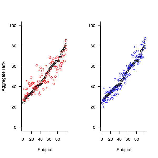
Figure 2. Aggregated ranking of snippets by subjects in years 1 and 2 (red and black) and years 2 and 4 (black and blue). Snippets have been sorted by year 2 ranking.
The above plot seems to show that at the aggregated year level there is much greater agreement between the 2nd/4th years than any other year pairing and measuring the correlation between each of the years using <Kendall’s tau>:
cs1.tau cs2.tau cs3.tau 0.6627602 0.6337914 0.8199636 |
confirms the greater agreement between this aggregate year pair.
Individual subject correlation to year aggregate ranking
To what extend to subject ratings correlate with their corresponding year aggregate? The following plot gives the correlation, using Kendall’s tau, between each subject and their corresponding year aggregate ranking.
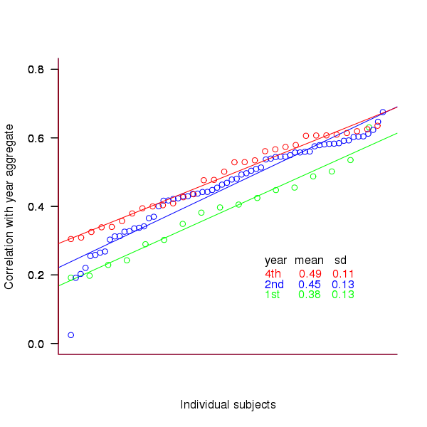
Figure 3. Correlation, using Kendall’s tau, between each subject and their corresponding year aggregate ranking.
The least squares fit shows that the variation in correlation across subjects in any year is very similar (removal of outliers in year 2 would make the lines almost parallel); the mean again shows a correlation that increases with year.
Discussion
The extent to which this study’s calculated values of rater agreement and correlation are considered worthy of further attention depends on the use to which the results will be put.
- From the perspective of trained raters the subject agreement in this study is very low and the rating have no further use.
- From the research perspective the results show that the concept of readability in the computer science student population has some non-zero substance to it that might be worth further study.
- From an overall perspective this study provides empirical evidence for a general lack of consensus on what constitutes readability.
It is not surprising that there is little agreement between student subjects on their readability rating, they are unlikely to have had much experience reading code and have not had any training in rating code for readability.
Professional developers will have spent years working with code and this experience is likely to have resulted in the creation of stable opinions on code readability. While developers usually work with code that is much longer than the few lines contained in the snippets used by Buse and Weimer, this experiment format is easy to administer and supports a fine level of control, i.e., allows a small set of source attributes of interest to be presented while excluding those not of interest. Repeating this study using such people as subjects would show whether this experience results in convergence to general agreement on the readability rating of code.
Summary of findings
The agreement between students readability ratings, for short snippets of code, improves as the students progress through course years 1 to 4 of a computer science degree.
While there is very good aggregated group agreement on the relative ranking of the readability of code snippets there is very little agreement between pairs of individuals.
- Two students chosen at random from within a year will have a low Spearman rank correlation coefficient for their rating of code snippet readability.
- Taken as a yearly aggregate there is a high degree of agreement between years two and four and less, but still good agreement between year 1 and other years.
- There is a broad range of correlations, from poor to good, between year aggregates and student subjects in the corresponding year.
Sequence generation with no duplicate pairs
Given a fixed set of items (say, 6 A, 12 B and 12 C) what algorithm will generate a randomised sequence containing all of these items with any adjacent pairs being different, e.g., no AA, BB or CC in the sequence? The answer would seem to be provided in my last post. However, turning this bit of theory into practice uncovered a few problems.
Before analyzing the transition matrix approach let’s look at some of the simpler methods that people might use. The most obvious method that springs to mind is to calculate the expected percentage of each item and randomly draw unused items based on these individual item percentages, if the drawn item matches the current end of sequence it is returned to the pool and another random draw is made. The following is an implementation in R:
seq_gen_rand_total=function(item_count) { last_item=0 rand_seq=NULL # Calculate each item's probability item_total=sum(item_count) item_prob=cumsum(item_count)/item_total while (sum(item_count) > 0) { # To recalculate on each iteration move the above two lines here. r_n=runif(1, 0, 1) new_item=which(r_n < item_prob)[1] # select an item if (new_item != last_item) # different from last item? { if (item_count[new_item] > 0) # are there any of these items left? { rand_seq=c(rand_seq, new_item) last_item=new_item item_count[new_item]=item_count[new_item]-1 } } else # Have we reached a state where a duplicate will always be generated? if ((length(which(item_count != 0)) == 1) & (which(item_count != 0)[1] == last_item)) return(0) } return(rand_seq) } |
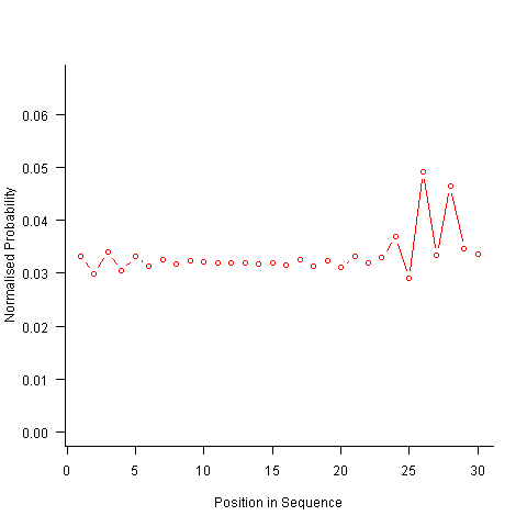
For instance, with 6 A, 12 B and 12 C, the expected probability is 0.2 for A, 0.4 for B and 0.4 for C. In practice if the last item drawn was a C then only an A or B can be selected and the effective probability of A is effectively increased to 0.3333. The red circles in the figure below show the normalised probability of an A appearing at different positions in the sequence of 30 items (averaged over 200,000 random sequences); ideally the normalised probability is 0.0333 for all positions in the sequence In practice the first position has the expected probability (there is no prior item to disturb the probability), the probability then jumps to a higher value and stays sort-of the same until the above-average usage cannot be sustained any more and there is a rapid decline (the sudden peak at position 29 is an end-of-sequence effect I talk about below).
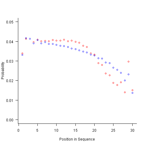
What might be done to get closer to the ideal behavior? A moments thought leads to the understanding that item probabilities change as the sequence is generated; perhaps recalculating item probabilities after each item is generated will improve things. In practice (see blue dots above) the first few items in the sequence have the same probabilities (the slight differences are due to the standard error in the samples) and then there is a sort-of consistent gradual decline driven by the initial above average usage (and some end-of-sequence effects again).
Any sequential generation approach based on random selection runs the risk of reaching a state where a duplicate has to be generated because only one kind of item remains unused (around 80% and 40% respectively for the above algorithms). If the transition matrix is calculated on every iteration it is possible to detect the case when a given item must be generated to prevent being left with unusable items later on. The case that needs to be checked for is when the percentage of one item is greater than 50% of the total available items, when this occurs that item must be generated next, e.g., given (1 A, 1 B, 3 C) a C must be generated if the final list is to have the no-pair property.
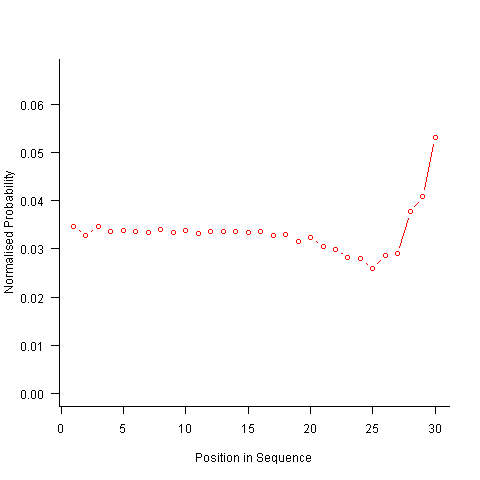
Now the transition matrix approach. Here the last item generated selects the matrix row and a randomly generated value selects the item within the row. Let’s start by generating the matrix once and always using it to select the next item; the resulting normalised probability stays constant for much longer because the probabilities in the transition matrix are not so high that items get used up early in the sequence. There is a small decline near the end and the end-of-sequence effects kick in sooner. Around 55% of generated sequences failed because two of the items were used up early leaving a sequence of duplicates of the remaining item at the end.
Finally, or so I thought, the sought after algorithm using a transition matrix that is recalculated after every item is generated. Where did that oscillation towards the end of the sequence come from?
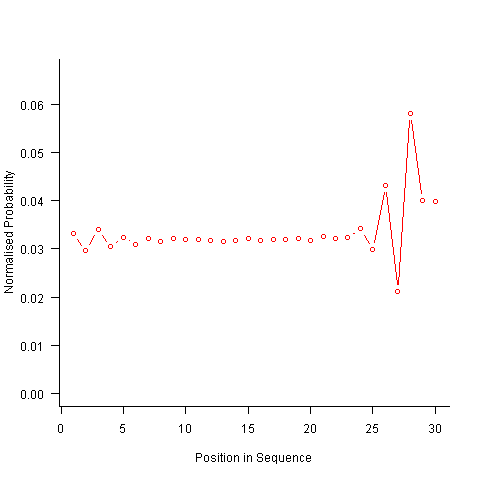
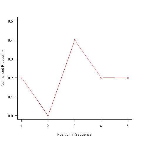
After a some head scratching I realised that the French & Perruchet algorithm is based on redistribution of the expected number of items pairs. Towards the end of the sequence there is a growing probability that the number of remaining As will have dropped to one; it is not possible to create an AA pair from only one A and the assumptions behind the transition matrix calculation break down. A good example of the consequences of this breakdown is the probability distribution for the five item sequences that the algorithm might generate from (1 A, 2 B, 2 C); an A will never appear in position 2 of the sequence:
After various false starts I decided to update the French & Perruchet algorithm to include and end-of-sequence state. This enabled me to adjust the average normalised probability of the main sequence (it has be just right to avoid excess/missing probability inflections at the end), but it did not help much with the oscillations in the last five items (it has to be said that my updated calculations involve a few hand-waving approximations of their own).
I found that a simple, ad hoc solution to damp down the oscillations is to increase any single item counts to somewhere around 1.3 to 1.4. More thought is needed here.
Are there other ways of generating sequences with the desired properties? French & Perruchet give one in their paper; this generates a random sequence, removes one item from any repeating pairs and then uses a random insert and shuffle algorithm to add back the removed items. Robert French responded very promptly to my queries about end-of-sequence effects, sending me a Matlab program implementing an updated version of the algorithm described in the original paper that he tells does not have this problem.
The advantage of the transition matrix approach is that the next item in the sequence can be generated on an as needed basis (provided the matrix is calculated on every iteration it is guaranteed to return a valid sequence if one exists; of course this recalculation removes some randomness for the sequence because what has gone before has some influence of the item distribution that follows). R code used for the above analysis.
I have not been able to locate any articles describing algorithms for generating sequences that are duplicate pair free and would be very interested to hear of any reader experiences.
Transition probabilities when adjacent sequence items must be different
Generating a random sequence from a fixed set of items is a common requirement, e.g., given the items A, B and C we might generate the sequence BACABCCBABC. Often the randomness is tempered by requirements such as each item having each item appear a given number of times in a sequence of a given length, e.g., in a random sequence of 100 items A appears 20 times, B 40 times and C 40 times. If there are rules about what pairs of items may appear in the sequence (e.g., no identical items adjacent to each other), then sequence generation starts to get a bit complicated.
Let’s say we want our sequence to contain: A 6 times, B 12 times and C 12 times, and no same item pairs to appear (i.e., no AA, BB or CC). The obvious solution is to use a transition matrix containing the probability of generating the next item to be added to the end of the sequence based on knowing the item currently at the end of the sequence.
My thinking goes as follows:
- given A was last generated there is an equal probability of it being followed by B or C,
- given B was last generated there is a 6/(6+12) probability of it being followed by A and a 12/(6+12) probability of it being followed by C,
- given C was last generated there is a 6/(6+12) probability of it being followed by A and a 12/(6+12) probability of it being followed by B.
giving the following transition matrix (this row by row approach having the obvious generalization to more items):
                 Second item
               A      B       C
          A    0     .5      .5
First
item      B   .33     0      .67

C .33 .67 0 |
Having read Generating constrained randomized sequences: Item frequency matters by Robert M. French and Pierre Perruchet (from whom I take these examples and algorithm on which the R code is based), I now know this algorithm for generating transition matrices is wrong. Before reading any further you might like to try and figure out why.
The key insight is that the number of XY pairs (reading the sequence left to right) must equal the number of YX pairs (reading right to left) where X and Y are different items from the fixed set (and sequence edge effects are ignored).
If we take the above matrix and multiply it by the number of each item we get the following (if A occurs 6 times it will be followed by B 3 times and C 3 times, if B occurs 12 times it will be followed by A 4 times and C 8 times, etc):
                 Second item
               A      B       C
          A    0      3       3
First
item      B    4      0       8

C 4 8 0 |
which implies the sequence will contain AB 3 times when counted forward and BA 4 times when counted backwards (and similarly for AC/CA). This cannot happen, the matrix is not internally consistent.
The correct numbers are:
                 Second item
               A      B       C
          A    0      3       3
First
item      B    3      0       9

C 3 9 0 |
giving the probability transition matrix:
                 Second item
               A      B       C
          A    0     .5      .5
First
item      B   .25     0      .75

C .25 .75 0 |
This kind of sequence generation occurs in testing and I wonder how many people have made the same mistake as me and scratched their heads over small deviations from the expected results.
The R code to calculate the transition matrix is straight forward but obscure unless you have the article to hand:
# Calculate expression (3) from: # Generating constrained randomized sequences: Item frequency matters # Robert M. French and Pierre Perruchet transition_count=function(item_count) { N_total=sum(item_count) # expected number of transitions ni_nj=(item_count %*% t(item_count))/(N_total-1) diag(ni_nj) = 0 # expected number of repeats d_k=item_count*(item_count-1)/(N_total-1) # Now juggle stuff around to put the repeats someplace else n=sum(ni_nj) n_k=rowSums(ni_nj) s_k=n - 2*n_k R_i=d_k / s_k R=sum(R_i) new_ij=ni_nj*(1-R) + (n_k %*% t(R_i)) + (R_i %*% t(n_k)) diag(new_ij)=0 return(new_ij) } transition_prob=function(item_count) { tc=transition_count(item_count) tp=tc / rowSums(tc) # relies on recycling return(tp) } |
the following calls:
transition_count(c(6, 12, 12)) transition_prob(c(6, 12, 12)) |
return the expected results.
French and Perruchet provide an Excel spreadsheet (note this contains a bug, the formula in cell F20 should start with F5 rather than F6).
Changes in optimization performance of gcc over time
The SPEC benchmarks came out a year after the first release of gcc (in fact gcc was and still is one of the programs included in the benchmark). Compiling the SPEC programs using the gcc option -O2 (sometimes -O3) has always been the way to measure gcc performance, but after 25 years does this way of doing things tell us anything useful?
The short answer: No
The longer answer is below as another draft section from my book Empirical software engineering with R book. As always comments welcome.
Changes in optimization performance of gcc over time
The GNU Compiler Collection <book gcc-man_12> (GCC) is under active development with its most well known component, the C compiler gcc, now over 25 years old. After such a long period of development is the quality of code generated by gcc still improving and if so at what rate? The method typically used to measure compiler performance is to compile the [SPEC] benchmarks with a small set of optimization options switched on (e.g., the O2 or O3 options) and this approach is used for the analysis performed here.
Data
Vladimir N. Makarow measured the performance of 9 releases of gcc, occurring between 2003 and 2010, on the same computer using the same benchmark suite (SPEC2000); this data is used in the following analysis.
The data contains the [SPEC number] (i.e., runtime performance) and code size measurements on 12 integer programs (11 in C and one in C+\+) from SPEC2000 compiled with gcc versions 3.2.3, 3.3.6, 3.4.6, 4.0.4, 4.1.2, 4.2.4, 4.3.1, 4.4.0 and 4.5.0 at optimization levels O2 and O3 (the mtune=pentium4 option was also used) 32-bit for the Intel Pentium 4 processor.
The same integer programs and 14 floating-point programs (10 in Fortran and 4 in C) were compiled for 64-bits, again with the O2 and O3 options (the mpc64 floating-point option was also used), using gcc versions 4.0.4, 4.1.2, 4.2.4, 4.3.1, 4.4.0 and 4.5.0.
Is the data believable?
The following are two fitness-for-purpose issues associated with using programs from SPEC2000 for these measurements:
-
the benchmark is designed for measuring processor performance not
compiler performance, -
many of its programs have been used for compiler benchmarking for
many years and it is likely that gcc has already been tuned to do
well on this benchmark.
The runtime performance measurements were obtained by running each programs once, SPEC requires that each program be run three times and the middle one chosen. Multiple measurements of each program would have increased confidence in their accuracy.
Predictions made in advance
Developers continue to make improvements to gcc and it is hoped that its optimization performance is increasing, knowing that performance is at a steady state or decreasing performance is also of interest.
No hypothesis is proposed for how optimization performance, as measured by the O2 and O3 options, might change between releases of gcc over the period 2003 to 2010.
The gcc documentation says that using the O3 option causes more optimizations to be performed than when the O2 option is used and therefore we would expect better performance for programs compiled with O3.
Applicable techniques
Modelling individual O2 and O3 option performance
One technique for modelling changes in optimization performance is to build a linear model that fits the gcc version (i.e., version is the predictor variable) to the average performance of the code it generate, calculating the averaged performance over each of the programs measured with the corresponding version of gcc. The problem with this approach is that by calculating an average it is throwing away information that is available about the variation in performance across different programs.
Building a [mixed-effects] model would make use of all the data when fitting a relationship between two quantities where there is a recurring random component (i.e., the SPEC program used). The optimizations made are likely to vary between different SPEC programs, we could treat the performance variations caused by difference in optimization as being random and having an impact on the mean performance value of all programs.
Programs differ in the magnitude of their SPEC number and code size, the measurements were converted to the percentage change compared against the values obtained using the earliest version of gcc in the measurement set.
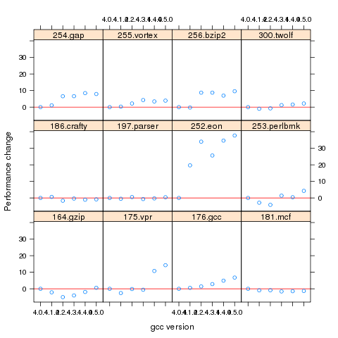
Figure 1. Percentage change in SPEC number (relative to version 4.0.4) for 12 programs compiled using 6 different versions of gcc (compiling to 64-bits with the O3 option).
Fitting a linear model requires at least two sets of [interval data]. The gcc version numbers are [ordinal values] and the following are two possible ways of mapping them to interval values:
-
there have been over 150 different released versions of gcc and a
particular version could be mapped to its place in this sequence. -
the date of release of a version can be mapped to the number of
days since the first release.
If version releases are organized around new functionality added then it makes sense to use version sequence number. If the performance of a new optimization was proportional to the amount of effort (e.g., man days) that went into its implementation then it would make sense to use days between releases.
The versions tested by Makarow were each from a different secondary release within a given primary version line and at roughly yearly intervals (two years separated the first pair and one month another pair).
There have been approximately 25 secondary releases in the 25 year project and using a release version sequence number starting at 20 seems like a reasonable choice.
Internally a compiler optimizer performs many different kinds of optimizations (gcc has over 160 different options for controlling machine independent optimization behavior). While the implementation of a new optimization is a gradual process involving many days of work, from the external user perspective it either exists and does its job when a given optimization level is supported or it does not exist.
What is the shape of the performance/release-version relationship? In the first few years of a compilers development it is to be expected that all the known major (i.e., big impact) optimization will be implemented and thereafter newly added optimizations have a progressively smaller impact on overall performance. Given gcc’s maturity it looks reasonable to assume that new releases contain a few additional improvement that have an incremental impact, i.e., the performance/release-version relationship is assumed to be linear (no other relationship springs out of a plot of the data).
A mixed-effects model can be created by calling the R function lme from the package nlme. The only difference between the following call to lme and a call to lm is the third argument specifying the random component.
t.lme=lme(value ~ variable, data=lme.O2, random = ~ 1 | Name) |
The argument random = ~ 1 | Name specifies that the random component effects the mean value of the result (when building a model this translates to an effect on the value of the intercept of the fitted equation) and that Name (of the program) is the grouped variable.
To specify that the random effect applies to the slope of the equation rather than its intercept the call is as follows:
t.lme=lme(value ~ variable, data=lme.O2, random = ~ variable -1 | Name) |
To specify that both the slope and the intercept are effected the -1 is omitted (for this gcc data the calculation fails to converge when both can be effected).
Since the measurements are about different versions of gcc it is to be expected that the data format has a separate column for each version of gcc (the format that would be used to pass data lm) as follows:
Name v3.2.3 v3.3.6 v3.4.6 v4.0.4 v4.1.2 v4.2.4 v4.3.1 v4.4.0 v4.5.0 1 164.gzip 933 932 957 922 933 939 917 969 955 2 175.vpr 562 561 577 576 586 585 576 589 588 3 176.gcc 1087 1084 1159 1135 1133 1102 1146 1189 1211 |
The relationship between the three variables in the call to lme is more complicated and the data needs to be reorganize so that one column contains all of the values, one the gcc version numbers and another column the program names. The function melt from package reshape2 can be used to restructure the data to look like:
Name variable value 11 256.bzip2 v3.2.3 0.000000 12 300.twolf v3.2.3 0.000000 13 SPECint2000 v3.2.3 0.000000 14 164.gzip v3.3.6 -0.107181 15 175.vpr v3.3.6 -0.177936 16 176.gcc v3.3.6 -0.275989 17 181.mcf v3.3.6 0.148810 |
Comparing O2 and O3 option performance
When comparing two samples the [Wilcoxon signed-rank test] and the [Mann-Whitney U test] spring to mind. However, some of the expected characteristics of the data violate some of the properties that these tests assume hold (e.g., every release include new/updated optimizations which is likely to result in the performance of each release having a different mean and variance).
The difference in performance between the two optimization levels could be treated as a set of values that could be modelled using the same techniques applied above. If the resulting model have a line than ran parallel with the x-axis and was within the appropriate confidence bounds we could claim that there was no measurable difference between the two options.
Results
The following is the output produced by summary for a mixed-effect model, with the random variation assumed to effect the value of intercept, created from the SPEC numbers for the integer programs compiled for 64-bit code at optimization level O2:
Linear mixed-effects model fit by REML
 Data: lme.O2
       AIC      BIC    logLik
  453.4221 462.4161 -222.7111

Random effects:
 Formula: ~1 | Name
        (Intercept) Residual
StdDev:    7.075923 4.358671

Fixed effects: value ~ variable
                 Value Std.Error DF   t-value p-value
(Intercept) -29.746927  7.375398 59 -4.033264   2e-04
variable      1.412632  0.300777 59  4.696612   0e+00
 Correlation:
         (Intr)
variable -0.958

Standardized Within-Group Residuals:
        Min          Q1         Med          Q3         Max
-4.68930170 -0.45549280 -0.03469526  0.31439727  2.45898648

Number of Observations: 72
Number of Groups: 12
|
and the following summary output is from a linear model built from an average of the data used above.
Call:
lm(formula = value ~ variable, data = lmO2)

Residuals:
      13       26       39       52       65       78
 0.16961 -0.32719  0.47820 -0.47819 -0.01751  0.17508

Coefficients:
             Estimate Std. Error t value Pr(>|t|)
(Intercept) -28.29676    2.22483  -12.72 0.000220 ***
variable      1.33939    0.09442   14.19 0.000143 ***
---
Signif. codes:  0 ‘***’ 0.001 ‘**’ 0.01 ‘*’ 0.05 ‘.’ 0.1 ‘ ’ 1

Residual standard error: 0.395 on 4 degrees of freedom
Multiple R-squared: 0.9805,     Adjusted R-squared: 0.9756
F-statistic: 201.2 on 1 and 4 DF,  p-value: 0.0001434
|
The biggest difference is that the fitted values for the Intercept and slope (the column name, variable, gives this value) have a standard error that is 3+ times greater for the mixed-effects model compared to the linear model based on using average values (a similar result is obtained if the mixed-effects random variation is assumed to effect the slope and the calculation fails to converge if the variation is on both intercept and slope). One consequence of building a linear model based on averaged values is that some of the variations present in the data are smoothed out. The mixed-effects model is more accurate in that it takes all variations present in the data into account.
For integer programs compiled for 32-bits there is much less difference between the mixed-effects models and linear models than is seen for 64-bit code.
-
For SPEC performance the created models show:
-
for the integer programs a rate of increase of around 0.6% (sd
0.2) per release forO2andO3options on 32-bit code
and an increase of 1.4% (sd 0.3) for 64-bit code, -
for floating-point, C programs only, a rate of increase per
release of 12% (sd 5) at 32-bits and 1.4% (sd 0.7) at 64-bits, with
very little difference between theO2andO3options.
-
for the integer programs a rate of increase of around 0.6% (sd
-
For size of generated code the created models show:
-
for integer programs 32-bit code built using
O2size is
decreasing at the rate of 0.6% (sd 0.1) per release, while for both
64-bit code andO3the size is increasing at between 0.7% (sd
0.2) and 2.5% (sd 0.4) per release, -
for floating-point, C programs only, 32-bit code built using
O2had an unacceptable p-value, while for both 64-bit code
andO3the size is increasing at between 1.6% (sd 0.3) and
9.3 (sd 1.1) per release.
-
for integer programs 32-bit code built using
Comparing O2 and O3 option performance
The intercept and slope values for the models built for the SPEC integer performance difference had p-values way too large to be of interest (a ballpark estimate of the values would suggest very little performance difference between the two options).
The program size change models showed O3 increasing, relative to O2, at 1.4% to 1.7% per release.
Discussion
The average rate of increase in SPEC number is very low and does not appear to be worth bothering about, possible reasons for this include:
-
a lot of effort has already been invested in making sure that gcc
performs well on the SPEC programs and the optimizations now being
added to gcc are aimed at programs having other kinds of
characteristics, -
gcc is a mature compiler that has implemented all of the worthwhile
optimizations and there are no more major improvements left to be
made, -
measurements based on just setting the
O2orO3
options might not provide a reliable guide to gcc optimization
performance. The command
gcc -c -Q -O2 --help=optimizers
shows that for gcc version 4.5.0 theO2option enables 91 of
the possible 174 optimization options and theO3option
enables 7 more. Performing some optimizations together sometimes
results in poorer quality code than if a subset of those
optimizations had been applied (genetic programming is being
researched as one technique for selecting the best optimizations
options to use for a given program and up to 13% improvements have
been obtained over gcc’s -O options <book Bashkansky_07>). The
percentage performance change figure above shows
that for some programs performance decreases on some releases.Whole program optimization is a major optimization area that has been addressed in recent versions of gcc, this optimizations is not enabled by the
Ooptions.
The percentage differences in SPEC integer performance between the O2 and O3 options were very small, but varied too much to be able to build a reliable linear model from the values.
For SPEC program code size there is a significant different between the O2 and O3 options. This is probably explained by function inlining being one of the seven additional optimization enabled by O3 (inlining multiple calls to the same function often increases code size <book inlining> and changes to the inlining optimization over releases could result in more functions being inlined).
Conclusion
Either the optimizations added to gcc between 2003 and 2010 have not made any significant difference to the performance of the generated code or the established method of measuring gcc optimization performance (i.e., the SPEC benchmarks and the O2 or O3 compiler options) is no longer a reliable indicator.
The most worthwhile R coding guidelines I know
Since my post questioning whether native R usage exists (e.g., a common set of R coding patterns) several people have asked about coding/style guidelines for R. My approach to style/coding guidelines is economic, adhering to a guideline involves paying a cost now for some future benefit. Obviously to be worthwhile the benefit must be greater than the cost, there is also the issue of who pays the cost and who reaps the benefit (why would anybody pay the cost if somebody else reaps the benefit?). The following three topics are probably where the biggest benefits are to be had and only the third is specific to R (and given the state of my R knowledge may be wrong).
Comment your code. Investing 5-10 seconds per few lines of code now could save substantially more time at some future date. Effective commenting is a skill that has to be learned, start learning now. Think of commenting as sending a text message or tweet to the person you will be in 6 months time (i.e., the person who can hum the tune but has forgotten the details).
Consistently use variable names that mean something to you. This should be a sub 2-second decision that is probably going to save you no more than 5-10 seconds, but in many cases you reap the benefit soon after the investment, without having to wait many months. Names evoke associations in your mind, take advantage of this associative lookup to reduce the cognitive load of working with your code. Effective naming is a skill that has to be learned, start learning now. There are people who ignore the evidence that different people’s linguistic preferences and associations can be very different and insist that everybody adhere to one particular naming convention; ignore them.
Code organization and structure. Experience shows that there are ways of organizing and structuring +1,000 line programs that have a significant impact on the effort needed to actively work on the code, the more code there is the greater the impact. R programs tend to be short, say around 100 lines (I dare say much longer ones exist). Apart from recommending that code be broken up into separate functions, I cannot think of any organizational/structural issue that is worth recommending for 100 lines of code (if you don’t appreciate the advantage of using separate functions you need some hands on training, not words in a blog post).
Is that it, are there no other worthwhile recommendations? There might be, I just don’t have enough experience using R to know. Does anybody else have enough experience to know? I suspect not; where would they have gotten the information needed to do the cost/benefit analysis? Even in the rare case where a detailed analysis is made for a language the results are rather thin on the ground and somewhat inconclusive.
What is the reason behind those R style guides/coding guideline documents that have been written? The following are some possibilities:
and no, I don’t have any empirical data to backup my guidelines 🙁