Archive
Occurrence of binary operator overloading in C++
Operator overloading, like many programming language constructs, was first supported in the 1960s (Algol 68 also provided a means to specify a precedence for the operator). C++ is perhaps the most widely used language supporting operator overloading; but not redefining their precedence.
I have always thought that operator overloading was more talked about than actually used (despite its long history, I have not been able to find any published usage information). A previous post noted that the CodeQL databases hosted by GitHub provides the data needed to measure usage, and having wrestled with the documentation (ql scripts used), C++ operator overload usage data is available.
The table below shows the total uses of overloaded and ‘usual’ binary operators in the source code (excluding headers) of 77 C++ repositories on GitHub (the 100 repositories C/C+ MRVA). The table is ordered by total occurrences of overloads, with the Percentage column showing the percentage use of overloaded operators against the total for the respective operator (i.e.,  ; code and data):
Binary Overload Usual Total Percentage << 103,855 20,463 124,318 83.5 == 21,845 118,037 139,882 15.6 != 14,749 69,273 84,022 17.6 * 12,849 57,906 70,755 18.2 + 10,928 103,072 114,000 9.6 && 8,183 64,148 72,331 11.3 - 5,064 77,775 82,839 6.1 <= 3,960 18,344 22,304 17.8 & 3,320 27,388 30,708 10.8 < 1,351 93,393 94,744 1.4 >> 1,082 11,038 12,120 8.9 / 1,062 29,023 30,085 3.5 > 537 44,556 45,093 1.2 >= 473 27,738 28,211 1.7 | 293 13,959 14,252 2.0 ^ 71 1,248 1,319 5.4 <=> 13 12 25 52.0 % 11 9,338 9,349 0.1 || 9 53,829 53,838 0.017 |
Use of the overloaded << operator is driven by standard library I/O, rather than left shifting.
There are seven operators where 10-20% of the usage is overloaded, which is a lot higher than I was expecting (not that I am a C++ expert).
How much does overloaded binary operator usage vary across projects? In the plot below, each vertical colored violin plot shows the distribution of overload usage for one operator across all 77 projects (the central black lines denote the range of the central 50% of the points; code and data):

While there is some variation between these 77 projects, in most cases a non-trivial percentage of an operator's usage is overloaded.
When task time measurements are not reported by developers
Measurements of the time taken to complete a software development task usually rely on the values reported by the person doing the work. People often give round number answers to numeric questions. This rounding has the effect of shifting start/stop/duration times to 5/10/15/20/30/45/60 minute boundaries.
To what extent do developers actually start/stop tasks on round number time boundaries, or aim to work for a particular duration?
The ABB Dev Interaction Data contains 7,812,872 interactions (e.g., clicking an icon) with Visual Studio by 144 professional developers performing an estimated 27,000 tasks over about 28,000 hours. The interaction start/stop times were obtained from the IDE to a 1-second resolution.
Completing a task in Visual Studio involves multiple interactions, and the task start/end times need to be extracted from each developer’s sequence of interactions. Looking at the data, rows containing the File.Exit message look like they are a reliable task-end delimiter (subsequent interactions usually happen many minutes after this message), with the next task for the corresponding developer starting with the next row of data.
Unfortunately, the time between two successive interactions is sometimes so long that it looks as if a task has ended without a File.Exit message being recorded. Plotting the number of occurrences of time-gaps between interactions (in minutes) suggests that it’s probably reasonable to treat anything longer than a 10-minute gap as the end of a task.
The plot below shows the number of tasks having a given duration, based on File.Exit, or using an 11-minute gap between interactions (blue/green) to indicate end-of-task, or a 20-minute gap (red; code+data):

The very prominent spikes in task counts at round numbers, seen in human reported times, are not present. The pattern of behavior is the same for both 11/20-minute gaps. I have no idea why there is a discontinuity at 10 minutes.
A development task is likely to involve multiple VS tasks. Is the duration of multiple VS tasks more likely to sum to a round number than a nonround number? There is no obvious reason why they should.
Is work on a VS task more likely to start/end at a round number time than a nonround number time?
Brief tasks are likely to be performed in the moment, i.e., without regard to clock time. Perhaps developers pay attention to clock time when tasks are expected to take some time.
The plot below shows the number of tasks taking at least 10-minutes that are started at a given number of minutes past the hour (blue/green), with red pluses showing 5-minute intervals (code+data):

No spikes in the count of tasks at round number start times (no spikes in the end times either; code+data).
Why spend time looking for round numbers where they are not expected to occur? Publishing negative results is extremely difficult, and so academics are unlikely to be interested in doing this analysis (not that software engineering researchers have shown any interest in round number usage).
The units of measurement for software reliability
How do the people define software reliability? One answer can be found by analyzing defect report logs: one study found that 42.6% of fault reports were requests for an enhancement, changes to documentation, or a refactoring request; a study of NASA spaceflight software found that 63% of reports in the defect tracking system were change requests.
Users can be thought of as broadly defining software reliability as the ability to support current (i.e., the software works as intended) and future needs (i.e., functionality that the user does not yet know they need, e.g., one reason I use R, rather than Python, for data analysis, is because I believe that if a new-to-me technique is required, a package+documentation supporting this technique is more likely to be available in R).
Focusing on current needs, the definition of software reliability depends on the perspective of who you ask, possibilities include:
- commercial management: software reliability is measured in terms of cost-risk, i.e., the likelihood of losing an amount £/$ as a result of undesirable application behavior (either losses from internal use, or customer related losses such as refunds, hot-line support, and good will),
- Open source: reliability has to be good enough and at least as good as comparable projects. The unit of reliability might be fault experiences per use of the program, or the number of undesirable behaviors encountered when processing pre-existing material,
- user-centric: mean time between failure per uses of the application, e.g., for a word processor, documents written/edited. For compilers, mean time between failure per million lines of source translated,
- academic and perhaps a generic development team: mean time between failure per million lines/instructions executed by the application. The definition avoids having to deal with how the software is used,
- available data: numeric answers require measurement data to feed into a calculation. Data that is relatively easy to collect is cpu time consumed by tests that found some number of faults, or perhaps wall time, or scraping the bottom of the barrel the number of tests run.
If an organization wants to increase software reliability, they can pay to make the changes that increase reliability. Pointing this fact out to people can make them very annoyed.
Sampling error in software engineering
In the physical sciences, measurement error occurs because of accuracy limits on the device used to make the measurement and the interpretation of the data by the person doing the measurement.
In software engineering, some measurements appear to be error free. For instance, lines of code is a discrete value that is easily counted. While some people don’t include blank lines and/or comments, the choice of what to count does not prevent an exact count being made.
In physics, the behavior of particular elements does not depend on the identity of which atoms are measured, while in software the behavior of programs written to the same specification can have different characteristics, e.g., lines of code.
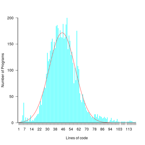
For instance, each implementation of the 3n+1 problem will contain some number of LOC, with other implementations often containing a different number of LOC. The plot below shows the distribution of LOC for 6,301 implementations of 3n+1 (code and data):

Each program implementing the 3n+1 problem is one sample from the population of programs implementing the 3n+1 specification. Different people are likely to implement different programs, and the same person may create different implementations at different times.
Sampling error occurs when the characteristics of a sample are used to infer characteristics about the population from which the sample was drawn.
How might sampling error affect the results of data analysis?
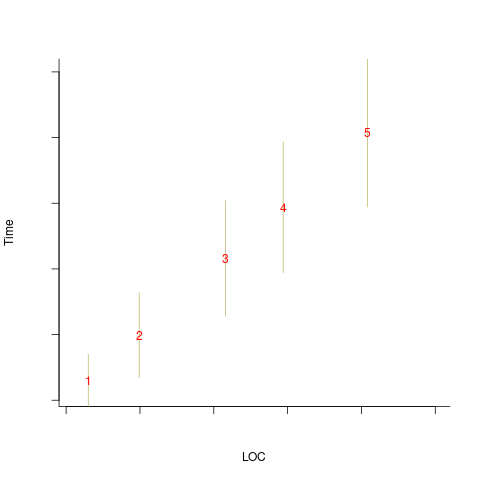
An example, using made-up values: Assume that two sets of sample measurements are made of the time taken to implement five different specifications, along with the lines of code contained in the implementations (in the same language). In the plot below, the yellow circles show a range of likely implementation measurements for each of the five specifications. The green dots, one for each specification, are measurements of one sample of programs implementing each specification; the blue dots are a second sample of programs (code):

The green and blue lines show the ordinary least squares regression model fitted to each sample. The different samples selected from the five populations has produced what appears to be slightly different models. How significant is this difference in the fitted models?
The grey line denotes where LOC is proportional to implementation time, which is one hypothesis of software project progress. The green line sample implies that LOC growth decreases as implementation time increases, while the blue line sample implies the reverse (both have been proposed as hypotheses of software project progress).
The difference in this example is important because the models fitted to the samples straddle the demarcation line between alternative theories of software project development.
A larger sample may not produce a more accurate model; a previous post analyses such a case. The example above shows a symmetric uniformly distributed population because that is the easiest to plot. In practice, populations distributions are likely to be asymmetric and irregular, e.g., measured time may be rounded to the nearest appropriate unit.
The mathematics underpinning OLS assumes that there is no error in the explanatory variables (LOC in the above plot), and that all the error is concentrated in the response variable (Time in the above plot). When there is a non-trivial sample error, or measurement error, OLS is not the appropriate technique to use to fit a regression model. The plot below shows the sample error that is assumed by OLS (code):

When there is a non-trivial error in the explanatory variable (LOC in this example), the appropriate technique for fitting a regression model is errors-in-variables regression.
Building an errors-in-variables regression model requires values for the error in the variables appearing in the equation to be fitted. Obtaining these values can be very difficult (Deming regression is a fitting technique based on the ratio of the errors).
In the above example, what is the likely variability in the implementation time and LOC, for a given specification? The limited data on the LOC contained in multiple implementations of the same specification suggests that the standard deviation of the LOC across implementations of the same specification is around 25% of the mean.
Learning researchers have run experiments where each subject performs the same task multiple times. Performance improves with practice, which makes it difficult to calculate the likely variability in the first-time performance.
My book: Evidence-based software engineering recommends using SIMEX to fit errors-in-variables models (section 11.2.3). This technique takes a model fitted using existing methods (allowing a wide range of models to be fitted), and then refits the model created based on the estimated error in one or more explanatory variables (no need to estimate an error in the response variable, the technique makes use of the value from the initial fit).
Number of parameters vs. accessing globals
I spend a lot of time looking at software engineering data, asking, what is the story here?
In a previous post I suggested that the distribution of the number of functions defined to have a given number of parameters, might be a signature of developer beliefs about the relative cost of parameter passing vs accessing globals.
Looking at the data that Iran Rodrigues Gonzaga Junior made available (good man), as part of his thesis Empirical Studies on Fine-Grained Feature Dependencies, I saw it contained information about the number of parameters in a function definition and whether functions accessed a global (Gonzaga’s research question is in another direction; I am always repurposing data).
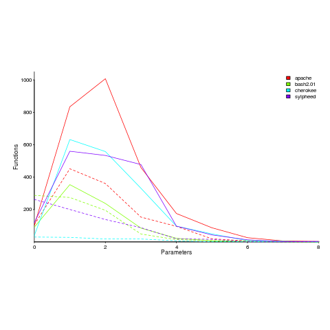
Are functions that access globals, defined with fewer parameters, compared to those that do not contain any such access? The plot below shows a count of the number of functions defined to have a given number of parameters, for four systems written in C; the solid lines are functions that did not access globals, the dashed lines are functions that accessed globals (code+data).

Over all 50 projects measured, functions that don’t access globals are defined, on average, to have an extra 0.7 parameters (the fitted Poisson regression models are better than a poke in the eye {i.e., the distribution is not really Poisson}, it’s more informative to look at the plotted data).
There is a lot of variation between projects (I picked these four because they were the larger projects and showed variation in behaviors). While the shape of the distributions varies a lot, there is always a noticeable difference in the mean.
Is this difference between projects a difference in developer beliefs, a difference in application requirements, a difference in developer coding habits (and parameter usage is a side effect; are there really that many getters and setters)?
I was hoping for a simple answer, and could not find one. Since I am writing a book and not researching individual issues in detail, it’s time to move on.
Ideas welcome.
Developers do not remember what code they have written
The size distribution of software components used in building many programs appears to follow a power law. Some researchers have and continue to do little more than fit a straight line to their measurements, while those that have proposed a process driving the behavior (e.g., information content) continue to rely on plenty of arm waving.
I have a very simple, and surprising, explanation for component size distribution following power law-like behavior; when writing new code developers ignore the surrounding context. To be a little more mathematical, I believe code written by developers has the following two statistical properties:
- nesting invariance. That is, the statistical characteristics of code sequences does not depend on how deeply nested the sequence is within
if/for/while/switchstatements, - independent of what went immediately before. That is the choice of what statement a developer writes next does not depend on the statements that precede it (alternatively there is no short range correlation).
Measurements of C source show that these two properties hold for some constructs in some circumstances (the measurements were originally made to serve a different purpose) and I have yet to see instances that significantly deviate from these properties.
How does writing code following these two properties generate a power law? The answer comes from the paper Power Laws for Monkeys Typing Randomly: The Case of Unequal Probabilities which proves that Zipf’s law like behavior (e.g., the frequency of any word used by some author is inversely proportional to its rank) would occur if the author were a monkey randomly typing on a keyboard.
To a good approximation every non-comment/blank line in a function body contains a single statement and statements do not often span multiple lines. We can view a function definition as being a sequence of statement kinds (e.g., each kind could be if/for/while/switch/assignment statement or an end-of-function terminator). The number of lines of code in a function is closely approximated by the length of this sequence.
The two statistical properties listed above allow us to treat the selection of which statement kind to write next in a function as mathematically equivalent to a monkey randomly typing on a keyboard. I am not suggesting that developers actually select statements at random, rather that the set of higher level requirements being turned into code are sufficiently different from each other that developers can and do write code having the properties listed.
Switching our unit of measurement from lines of code to number of tokens does not change much. Every statement has a few common forms that occur most of the time (e.g., most function calls contain no parameters and most assignment statements assign a scalar variable to another scalar variable) and there is a strong correlation between lines of code and token count.
What about object-oriented code, do developers follow the same pattern of behavior when creating classes? I am not aware of any set of measurements that might help answer this question, but there have been some measurements of Java that have power law-like behavior for some OO features.
Using third party measurement data
Until today, to the best of my knowledge, all the source code analysis papers I have read were written by researchers who had control of the code analysis tools they used and had some form of localised access to the source. By control of the code analysis tools I mean that the researchers specified the tool options and had the ability to check the behavior of the tool, in many cases the source of the tool was available to them and often even written by them, and the localised access may have involved downloading lots of code from the web.
I have just been reading about a broad brush analysis of comment usage based on data provided by a commercial code repository that offers API access to some basic code metrics.
At first, I was very frustrated by the lack of depth to the analysis provided in the paper, but then I realised that the authors’ intent was to investigate a few broad ideas about comment usage in a large number of projects (around 10,000). The authors complained in their blog about some of the referees comments and having to submit a shorter paper. I can see where the referees are coming from, the papers are lacking in depth of analysis, but they do contain some interesting results.
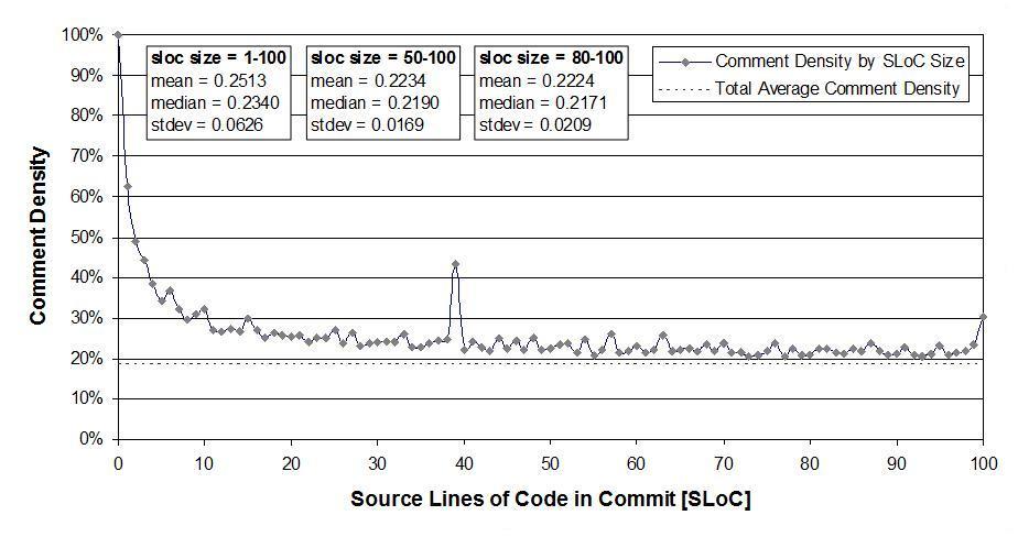
I was very interested in Figure 2:

which plots the comment density of the lines in a source code commit. I would expect the ratio to be higher for small commits because a developer probably has a relatively fixed amount to say about updates involving a smallish number of lines (which probably fixes a problem). Larger commits are probably updated functionality and so would have a comment density similar to the ‘average’.
The problem with relying on third parties to supply the data is that obtaining the answers to follow up questions invariably involves lots of work, e.g., creating an environment to perform the measurements needed for the follow-up questions. However, the third party approach can significantly reduce the amount of work needed to get to a point where the interestingness of the results can be gauged.