Archive
Modelling time to next reported fault
After the arrival of a fault report for a program, what is the expected elapsed time until the next fault report arrives (assuming that the report relates to a coding mistake and is not a request for enhancement or something the user did wrong, and the number of active users remains the same and the program is not changed)? Here, elapsed time is a proxy for amount of program usage.
Measurements (here and here) show a consistent pattern in the elapsed time of duplicate reports of individual faults. Plotting the time elapsed between the first report and the n’th report of the same fault in the order they were reported produces an exponential line (there are often changes in the slope of this line). For example, the plot below shows 10 unique faults (different colors), the number of days between the first report and all subsequent reports of the same fault (plus character); note the log scale y-axis (discussed in this post; code+data):

The first person to report a fault may experience the same fault many times. However, they only get to submit one report. Also, some people may experience the fault and not submit a report.
If the first reporter had not submitted a report, then the time of first report would be later. Also, the time of first report could have been earlier, had somebody experienced it earlier and chosen to submit a report.
The subpopulation of users who both experience a fault and report it, decreases over time. An influx of new users is likely to cause a jump in the rate of submission of reports for previously reported faults.
It is possible to use the information on known reported faults to build a probability model for the elapsed time between the last reported known fault and the next reported known fault (time to next reported unknown fault is covered at the end of this post).
The arrival of reports for each distinct fault can be modelled as a Poisson process. The time between events in a Poisson process with rate  has an exponential distribution, with mean
  . The distribution of a sum of multiple Poisson processes is itself a Poisson process whose rate is the sum of the individual rates. The other key point is that this process is memoryless. That is, the elapsed time of any report has no impact on the elapsed time of any other report.
If there are  different faults whose fitted report time exponents are:
  ,
,  …
…  , then summing the Poisson rates,
  , gives the mean
  , for a probability model of the estimated time to next any-known fault report.
To summarise. Given enough duplicate reports for each fault, it’s possible to build a probability model for the time to next known fault.
In practice, people are often most interested in the time to the first report of a previous unreported fault.
tl;dr Modelling time to next previously unreported fault has an analytic solution that depends on variables whose values have to be approximately approximated.
The method used to build a probability model of reports of known fault can be used extended to build a probability model of first reports of currently unknown faults. To build this model, good enough values for the following quantities are needed:
- the number of unknown faults,
 , remaining in the program. I have some ideas about estimating the number of unknown faults, , and will discuss them in another post,
 - the time,
 , needed to have received at least one report for each of the unknown faults. In practice, this is the lifetime of the program, and there is data on software half-life. However, all coding mistakes could trigger a fault report, but not all coding mistakes will have done so during a program’s lifetime. This is a complication that needs some thought,
 - the values of
 ,
,  …
…  for each of the unknown faults. There is some data suggesting that these values are drawn from an exponential distribution, or something close to one. Also, an equation can be fitted to the values of the known faults. The analysis below assumes that the
  for each unknown fault that might be reported is randomly drawn from an exponential distribution whose mean is .
This rate will be affected by program usage (i.e., number of users and the activities they perform), and source code characteristics such as the number of executions paths that are dependent on rarely true conditions.
Putting it all together, the following is the question I asked various LLMs (which uses  , rather than ):
There are independent processes. Each process,  , transmits a signal, and the number of signals transmitted in a fixed time interval, , has a Poisson distribution with mean
  for
for  . The values are randomly drawn from the same exponential distribution. What is the cumulative distribution for the time between the successive first signals from the processes.
The cumulative distribution gives the probability that an event has occurred within a given amount of time, in this case the time since the last fault report.
The ChatGPT 5.2 Thinking response (Grok Thinking gives the same formula, but no chain of thought): The probability that the  unknown fault is reported within time
  of the previous report of an unknown fault,
 ") , is given by the following rather involved formula:
, is given by the following rather involved formula:
=1-(a/{a+t})^{N-k}{}_{2}F_1(N-k, k; N+1; t/{a+t})")
where: is the initial number of faults that have not been reported,  , and
, and  is the hypergeometric function.
The important points to note are: the value  decreases as more unknown faults are reported, and the dominant contribution of the value .
Deepseek’s response also makes complicated use of the same variables, and the analysis is very similar before making some simplifications that don’t look right (text of response). Kimi’s response is usually very good, but for this question failed to handle the consequences of .
Almost all published papers on fault prediction ignore the impact of number of users on reported faults, and that report time for each distinct fault has a distinct distribution, i.e., their analysis is not connected to reality.
Lifetime of coding mistakes in the Linux kernel
What is the lifetime of coding mistakes in the Linux kernel? Some coding mistakes result in fault reports (some of which are fixed), while many are removed when the source that contains them is deleted/changed during ongoing development.
After fixing the coding mistake(s) in the kernel that generated a reported fault, developer(s) log the commit that introduced the coding mistake, along with the commit that fixed it. This logging started in 2013, and I only found out about it this week. To be exact, I discovered the repo: A dataset of Linux Kernel commits created by Maes Bermejo, Gonzalez-Barahona, Gallego, and Robles.
The log contains the commit hashes for the 90,760 fixes made to the 63 mainline kernel versions from 3.12 to 6.13. The complete log of 1,233,421 commits has to be searched to extract the details, e.g., date, lines added, etc.
The kernel development process involves regular release cycles of around 80 days. Developers submit the code they want to be included in the next release, this goes through a series of reviews, with Linus making the final decision.
The following analysis is based on the coding mistakes introduced between successive kernel releases, e.g., version 3.13 coding mistakes are those introduced into the source between 4 Nov 2013 (the day after version 3.12 was released) and 19 Jan 2014 (when version 3.13 was released). Code will have been worked on, and mistakes created/fixed, before it reached the kernel, which ensures some level of maturity.
The number of people working with pre-release code is likely to be tiny, compared to the number running released kernels. Consequently, the characteristics of coding mistake lifetime is expected to be different pre/post release, if only because more users are likely to report more faults.
The plot below shows the pre-release daily mistake fixed density against days since start of work on the current release, the red line is a fitted regression line mapped to density (fitted regression is a biexponential; code and data):
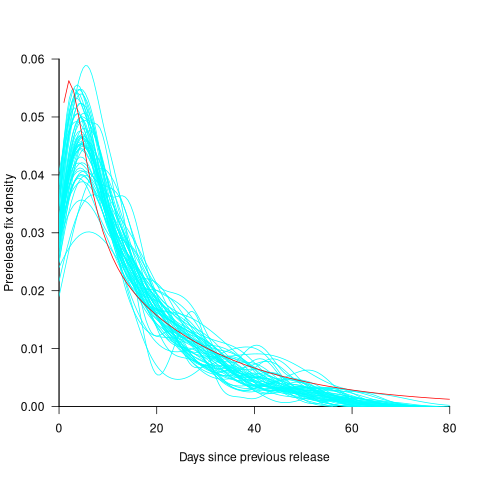
For all versions, the prior to release daily fix rate follows a consistent pattern: Most fixes occur in the first few days, with roughly an exponential decline to the release date.
The following analysis builds a broad brush model of cumulative fixes over time across 53 mainline kernel releases (the final 10 releases were not included because of their relatively short history).
The number of users of a new kernel takes time to increase as it percolates onto systems, e.g., adopted by Linux distributions and then installed by users, or installed by cloud providers. Eventually, code first included in a particular version will be running on most systems.
The post release daily fix rate is best modelled using the cumulative number of fixes, i.e., total number of fixes up to a given day since release. The models fitted below are based on dividing the post release cumulative fixes into before/after 200 days since release. The 200-day division is a round number (technically, a nearby value may provide a better fit) that supports the fitting of good quality before/after regression models. Averaged over all releases, 42% of fixes occurred within 200-days, and 58% after 200-days.
The plot below shows the cumulative number of post-release fixed faults, in red, for various kernel versions, with fitted regression lines in green and blue (grey line is at 200-days; code and data):

The equation fitted to the before 200-days fixes had the following form:
}")
where:  is a kernel version specific constant; see plot below.
The equation fitted to the after 200-days fixes had the following form:

where:  is a kernel version specific constant; see plot below.
Approximately, after release, the cumulative fix rate starts out quadratic in elapsed days, with the rate decreasing over time, until after 200-days the rate settles down to following the cube-root of days.
Comparing the number of post-release fixes across versions, there is a lot more variability in the first 200-days (i.e., the model fit to the data is sometimes very poor), relatively to after 200-days (where the model fit is consistently good).
Each kernel release has its own characteristics, parameterised by the values , and in the above equations. The plot below shows these values across versions, with red for , blue/green for , and grey line showing normalised LOC added/changed in the release (code and data):
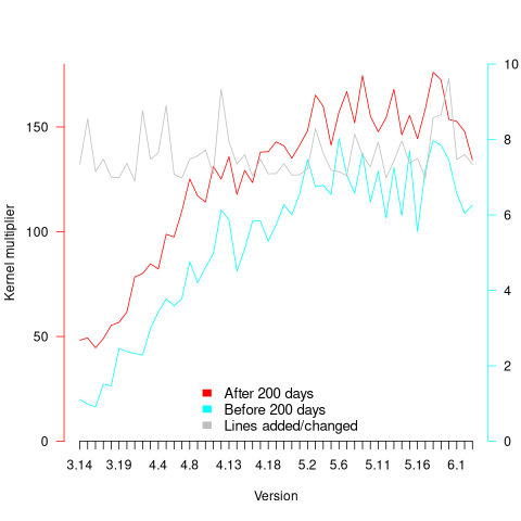
The plot clearly shows a large increase in the number of fixes between kernel version 3.14 and later versions. The before 200-days rate (blue/green) increase by a factor of seven, while the after 200-days rate increased by a factor of three.
Is this increase driven by some underlying factor in kernel development, or is it an external factor such as an increase in the number of users (more users leads to more faults reports), or the extensive post-release fuzz testing that is now common.
The number of lines of code added/changed, indicated by the grey line (shifted to fit plot axes) cannot be added to the fitted models because they exactly correlate with their respective version.
What is driving the long-term rate of fixes, i.e., cube-root of elapsed days?
Actually, what people are really want to know is what can be done to reduce the number of fixes required after release. When people ask me this, my usual reply is: “Spend more on testing”.
The probability of a coding mistake causing a fault report is decreasing: fixes reduce the number of remaining mistakes, and source added in one kernel version may be removed in a later version.
Perhaps the set of input behaviors is growing, producing the distinct conditions needed to trigger different coding mistakes, or the faults are occurring but are only reported when experienced by a small subset of users.
As always, more data is needed.
Percentage of methods containing no reported faults
It is often said, with some evidence, that 80% of reported faults, for a program, occur in 20% of its code. I think this pattern is a consequence of 20% of the code being executed 80% of the time, while many researchers believe that 20% of the source code has characteristics that result in it containing 80% of the coding mistakes.
The 20% figure is commonly measured as a percentage of methods/functions, rather than a percentage of lines of code.
This post investigates the expected fraction of a program’s methods that remain fault report free, based on two probability models.
Both models assume that coding mistakes are uniformly scattered throughout the code (i.e., every statement has the same probability of containing a mistake) and that the corresponding coding mistake is contained within a single method (the evidence suggests that this is true for 50% of faults).
A simple model is to assume that when a new fault is reported, the probability that the corresponding coding mistake appears in a particular method is proportional to the method’s length,  in lines of code, of the method. The evidence shows that the distribution of methods containing a given number of lines, , is well-fitted by a power law (for Java:
  ).
).
If  reported faults have been fixed in a program containing
  methods/functions, what is the expected number of methods that have not been modified by the fixing process?
The answer (with help from: mostly Kimi, with occasional help from Deepseek (who don’t have a share chat options), ChatGPT 5, Grok, and some approximations; chat logs) is:
}Li_b(e^{-{F/M}{{zeta(b)}/{zeta(b-1)}}})")
where:  is the Riemann zeta function,
  is the polylogarithm function and
  for Java.
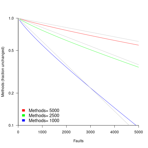
The plot below shows the predicted fraction of unmodified methods against number of faults, for programs of various sizes; the grey lines show the rough approximation:  (code+data):
The observed behavior of most reported faults involving a subset of a program’s methods can be modelled using some form of preferential attachment.
One preferential attachment model specifies that the likelihood of a coding mistake appearing in a method is proportional to ") , where
, where  is the number of previously detected coding mistakes in the method.
The estimated number of unmodified methods is now:
}Li_b(({M zeta(b-1)}/{M zeta(b-1)+a*(F+1) zeta(b)})^{1/a})")
where:  is the average value of
  over all faults (if
  , then
  for a power law with exponent 2.35).
The plot below shows the predicted fraction of unmodified methods against number of faults for a program containing 1,000 methods, for various values of , with the black line showing the fraction of unmodified methods predicted by the simple model above (code+data):
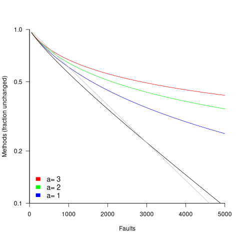
In practice, random selection of the method containing a coding mistake will introduce some fuzziness in the predicted fraction of unmodified methods.
As the number of reported faults grows, the attraction of methods involved in previous reported faults slows the rate at which methods experience their first detected coding mistake.
How realistic are these models?
By focusing on the number of unmodified methods, many complications are avoided.
Both models assume that an unchanging number of methods in a program and that the length of each method is fixed. This assumption holds between each release of a program.
For actively maintained programs, the number of methods in a program changes over time, and the length of some existing methods also changes (if a program were not actively maintained, reported faults would not get fixed).
These models are unlikely to be applicable to programs with short release cycles, where there are few reported faults between releases.
How well do the models’ predictions agree with the data?
At the moment, I am not aware of a dataset containing the appropriate data. Number of faults vs unmodified methods has been added to my list of interesting patterns to notice.
Summary of the derivation of the solutions for the two models.
Simple model
The expected number of unmodified methods, ") , is:
, is:
=sum{L=1}{T}{m_L{P(U_LF)}}") , where is the length of the longest method,
, where is the length of the longest method,  is the number of methods of length , and
 ") is the probability that a method of length will be unmodified after fault reports.
is the probability that a method of length will be unmodified after fault reports.
The evidence shows that the distribution of methods containing a given number of lines, , is well-fitted by a power law (for Java: ).
Given a program containing methods, the number of methods of length is:
 , where for Java.
If is large and  , then the sum can be approximated by the Riemann zeta function, , giving:
}}")
The probability that a method containing lines will not be modified by a fault report (assuming that fixing the mistake only involves one method) is:  , where
  is the total lines of code in the program, and the probability of this method not being modified after fault reports is approximately:
^F approx e^{{-F*L}/{P_t}}")
The expected number of empty boxes is:
}}*e^{{-F*L}/{P_t}}}=M/{zeta(b)}Li_b(e^{-F/{P_t}})")
The number of lines of code in a program containing methods is:
}}}=M/{zeta(b)}sum{L=1}{T}{L^{1-b}}=M{{zeta(b-1)}/{zeta(b)}}")
Finally giving:
}Li_b(e^{-{F/M}{{zeta(b)}/{zeta(b-1)}}})")
where is the polylogarithm function.
This equation is roughly, for the purposes of understanding the effect of each variable:

Preferential attachment model
When a mistake is corrected in a method, the attraction weight of that method increases (alternatively, the attraction weight of the other methods decreases). The probability that a method is not modified after fault reports is now:
}=prod{k=0}{F}{{P_t+a*k-L}/{P_t+a*k}}={Gamma({P_t}/a)Gamma({P_t-L}/a+F+1)}/{Gamma({P_t-L}/a)Gamma(P_t/a+F+1)}")
where:  the average value of over all faults, and
  is the gamma function.
applying the Stirling/Gamma–ratio rule, i.e., }/{Gamma(z+b)} approx z^{a-b}") we get:
we get:
})^{F/a} = ((P_t/{P_t+a*(F+1)})^{1/a})^F")
where the expression ^{1/a})^F") is the preferential attachment version of the expression
is the preferential attachment version of the expression ^F") appearing in the simple model derivation. Using this preferential attachment expression in the analysis of the simple model, we get:
appearing in the simple model derivation. Using this preferential attachment expression in the analysis of the simple model, we get:
I don’t have a rough approximation for this expression.
Deep dive looking for good enough reliability models
A previous post summarised the main highlights of my trawl through the software reliability research papers/reports/data, which failed to find any good enough models for estimating the reliability of a software system. This post summarises a deep dive into the technical aspects of the research papers.
I am now a lot more confident that better than worst case models for calculating software reliability don’t yet exist (perhaps the problem does not have a solution). By reliability, I mean the likelihood that a fault will be experienced during 1-hour of operation (1-hour is the time interval often used in safety critical standards).
All the papers assume that time to next new fault experience can be effectively modelled using timing information on the previously discovered distinct faults. Timing information might be cpu time, or elapsed time during testing or customer use, or even number of tests. Issues of code coverage and the correspondence between tests and customer usage are rarely mentioned.
Building a model requires making assumptions about the world. Given the data used, all the models assume that there is a relationship connecting the time between successive distinct faults, e,g, the Jelinski-Moranda model assumes that the time between fault experiences has an exponential distribution and that the exponent is the same for all faults. While the Jelinski-Moranda model does not match the behavior seen in the available datasets, it is widely discussed (its simplicity makes it a great example, with the analysis being straightforward and the result easy to explain).
Much of the fault timing data comes from the test process, with the rest coming from customer usage (either cpu or elapsed; like today’s cloud usage, mainframe time usage was often charged). What connection does a model fitted to data on the faults discovered during testing have with faults experienced by customers using the software? Managers want to minimise the cost of testing (one claimed use case for these models is estimating the likelihood of discovering a new fault during testing), and maximising the number of faults found probably has a higher priority than mimicking customer usage.
The early software reliability papers (i.e., the 1970s) invariably proposed a new model and then checked how well it fitted a small dataset.
While the top, must-read paper on software fault analysis was published in 1982, it has mostly remained unknown/ignored (it appeared as a NASA report written by non-academics who did not then promote their work). Perhaps if Nagel and Skrivan’s work had become widely known, today we might have a practical software reliability model.
Reliability research in the 1980s was dominated by theoretical analysis of the previously proposed models and their variants, finding connections between them and building more general models. Ramos’s 2009 PhD thesis contains a great overview of popular (academic) reliability models, their interconnections, and using them to calculate a number.
I did discover some good news. Researchers outside of software engineering have been studying a non-software problem whose characteristics have a direct mapping to software reliability. This non-software problem involves sampling from a population containing subpopulations of varying sizes (warning: heavy-duty maths), e.g., oil companies searching for new oil fields of unknown sizes. It looks, perhaps (the maths is very hard going), as-if the statisticians studying this problem have found some viable solutions. If I’m lucky, I will find a package implementing the technical details, or find a gentle introduction. Perhaps this thread will have a happy ending…
An aside: When quickly deciding whether a research paper is worth reading, if the title or abstract contains a word on my ignore list, the paper is ignored. One consequence of this recent detailed analysis is that the term NHPP has been added to my ignore list for software reliability issues (it has applicability for hardware).
Example of an initial analysis of some new NASA data
For the last 20 years, the bug report databases of Open source projects have been almost the exclusive supplier of fault reports to the research community. Which, if any, of the research results are applicable to commercial projects (given the volunteer nature of most Open source projects and that anybody can submit a report)?
The only way to find out if Open source patterns are present in closed source projects is to analyse fault reports from closed source projects.
The recent paper Software Defect Discovery and Resolution Modeling incorporating Severity by Nafreen, Shi and Fiondella caught my attention for several reasons. It does non-trivial statistical analysis (most software engineering research uses simplistic techniques), it is a recent dataset (i.e., might still be available), and the data is from a NASA project (I have long assumed that NASA is more likely than most to reliable track reported issues). Lance Fiondella kindly sent me a copy of the data (paper giving more details about the data)!
Over the years, researchers have emailed me several hundred datasets. This NASA data arrived at the start of the week, and this post is an example of the kind of initial analysis I do before emailing any questions to the authors (Lance offered to answer questions, and even included two former students in his email).
It’s only worth emailing for data when there looks to be a reasonable amount (tiny samples are rarely interesting) of a kind of data that I don’t already have lots of.
This data is fault reports on software produced by NASA, a very rare sample. The 1,934 reports were created during the development and testing of software for a space mission (which launched some time before 2016).
For Open source projects, it’s long been known that many (40%) reported faults are actually requests for enhancements. Is this a consequence of allowing anybody to submit a fault report? It appears not. In this NASA dataset, 63% of the fault reports are change requests.
This data does not include any information on the amount of runtime usage of the software, so it is not possible to estimate the reliability of the software.
Software development practices vary a lot between organizations, and organizational information is often embedded in the data. Ideally, somebody familiar with the work processes that produced the data is available to answer questions, e.g., the SiP estimation dataset.
Dates form the bulk of this data, i.e., the date on which the report entered a given phase (expressed in days since a nominal start date). Experienced developers could probably guess from the column names the work performed in each phase; see list below:
    Date Created
    Date Assigned
    Date Build Integration
    Date Canceled
    Date Closed
    Date Closed With Defect
    Date In Test
    Date In Work
    Date on Hold
    Date Ready For Closure
    Date Ready For Test
    Date Test Completed
Date Work Completed |
There are probably lots of details that somebody familiar with the process would know.
What might this date information tell us? The paper cited had fitted a Cox proportional hazard model to predict fault fix time. I might try to fit a multi-state survival model.
In a priority queue, task waiting times follow a power law, while randomly selecting an item from a non-prioritized queue produces exponential waiting times. The plot below shows the number of reports taking a given amount of time (days elapsed rounded to weeks) from being assigned to build-integration, for reports at three severity levels, with fitted exponential regression lines (code+data):
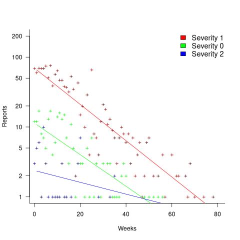
Fitting an exponential, rather than a power law, suggests that the report to handle next is effectively selected at random, i.e., reports are not in a priority queue. The number of severity 2 reports is not large enough for there to be a significant regression fit.
I now have some familiarity with the data and have spotted a pattern that may be of interest (or those involved are already aware of the random selection process).
As always, reader suggestions welcome.
Extracting information from duplicate fault reports
Duplicate fault reports (that is, reports whose cause is the same underlying coding mistake) are an underused source of information. I sometimes email the authors of a paper analysing fault data asking for information about duplicates. Duplicate information is rarely available, because the authors don’t bother to record it.
If a program’s coding mistakes are a closed population, i.e., no new ones are added or existing ones fixed, duplicate counts might be used to estimate the number of remaining mistakes.
However, coding mistakes in production software systems are invariably open populations, i.e., reported faults are fixed, and new functionality (containing new coding mistakes) is added.
A dataset made available by Sadat, Bener, and Miranskyy contains 18 years worth of information on duplicate fault reports in Apache, Eclipse and KDE. The following analysis uses the KDE data.
Fault reports are created by users, and changes in the rate of reports whose root cause is the same coding mistake provides information on changes in the number of active users, or changes in the functionality executed by the active users. The plot below shows, for 10 unique faults (different colors), the number of days between the first report and all subsequent reports of the same fault (plus character); note the log scale y-axis (code+data):
Changes in the rate at which duplicates are reported are visible as changes in the slope of each line formed by plus signs of the respective color. Possible reasons for the change include: the coding mistake appears in a new release which users do not widely install for some time, 2) a fault become sufficiently well known, or workaround provided, that the rate of reporting for that fault declines. Of course, only some fault experiences are ever reported.
Almost all books/papers on software reliability that model the occurrence of fault experiences treat them as-if they were a Non-Homogeneous Poisson Process (NHPP); in most cases, authors are simply repeating what they have read elsewhere.
Some important assumptions made by NHPP models do not apply to software faults. For instance, NHPP models assume that the probability of encountering a fault experience is the same for different coding mistakes, i.e., they are all equally likely. What does the evidence show about this assumption? If all coding mistakes had the same probability of producing a fault experience, the mean time between duplicate fault reports would be the same for all fault reports. The plot below shows the interval, in days, between consecutive duplicate fault reports, for the 392 faults whose number of duplicates was between 20 and 100, sorted by interval (out of a total of 30,377; code+data):
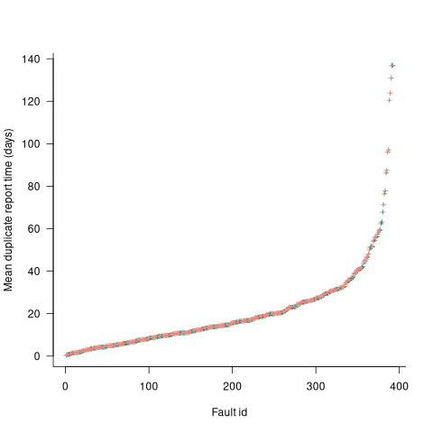
The variation in mean time between duplicate fault reports, for different faults, is evidence that different coding mistakes have different probabilities of producing a fault experience. This behavior is consistent with the observation that mistakes in deeply nested if-statements are less likely to be executed than mistakes contained in less-deeply nested code. However, this observation invalidating assumptions made by NHPP models has not prevented them dominating the research literature.
Good enough reliability models: still an unknown
Estimating the likelihood that a software system will operate as intended, for some period of time, is one of the big problems within the field of software reliability research. When software does not operate as intended, a fault, or bug, or hallucination is said to have occurred.
Three events need to occur for a user of a software system to experience a fault:
- a developer writes code that does not always behave as intended, i.e., a coding mistake,
- the user of the software feeds it input that causes the coding mistake to produce unintended behavior,
- the unintended behavior percolates through the system to produce a visible fault (sometimes an unintended behavior does not percolate very far, and does not produce any change of visible behavior).
Modelling each kind of event and their interaction is a huge undertaking. Researchers in one of the major subfields of software reliability take a global approach, e.g., they model time to next fault experience, using data on the number of faults experienced per given amount of cpu/elapsed time (often obtained during testing). Modelling the fault data obtained during testing results in a model of the likelihood of the next fault experienced using that particular test process. This is useful for doing a return-on-investment calculation to decide whether to do more testing. If the distribution of inputs used during testing is similar to the distribution of customer inputs, then the model can be of use in estimating the rate of customer fault experiences.
Is it possible to use a model whose design was driven by data from testing one or more software systems to estimate the rate of fault experiences likely when testing other software systems?
The number of coding mistakes will differ between systems (because they have different sizes, and/or different developer abilities), and the testers’ ability will be different, and the extent to which mistaken behavior percolates through code will differ. However, it is possible for there to be a general model for rate of fault experiences that contains various parameters that need to be fitted for each situation.
Since that start of the 1970s, researchers have been searching for this general model (the first software reliability model is thought to be: “Program errors as a birth-and-death process” by G. R. Hudson, Report SP-3011, System Development Corp., 1967 Dec 4; please send me a copy, if you have one).
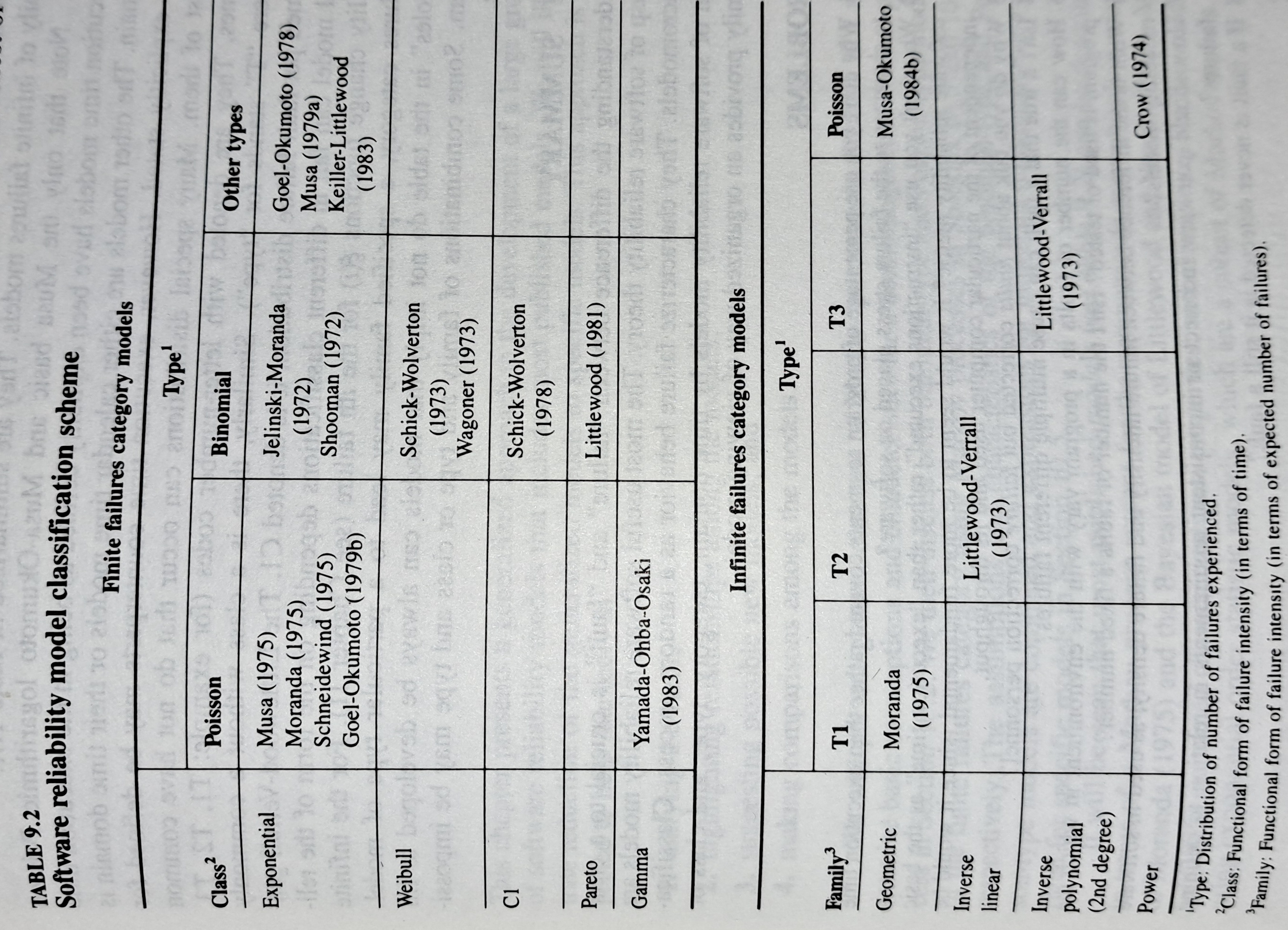
The image below shows the 18 models discussed in the 1987 book “Software Reliability: Measurement, Prediction, Application” by Musa, Iannino, and Okumoto (later editions have seriously watered down the technical contents, and lack most of the tables/plots). It’s to be expected that during the early years of a new field, many different models will be proposed and discussed.
Did researchers discover a good-enough general model for rate of fault experiences?
It’s hard to say. There is not enough reliability data to be confident that any of the umpteen proposed models is consistently better at predicting than any other. I believe that the evidence-based state of the art has not yet progressed beyond the 1982 report Software Reliability: Repetitive Run Experimentation and Modeling by Nagel and Skrivan.
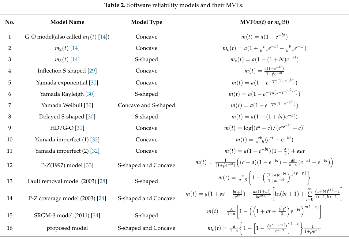
Fitting slightly modified versions of existing models to a small number of tiny datasets has become standard practice in this corner of software engineering research (the same pattern of behavior has occurred in software effort estimation). The image below shows 16 models from a 2021 paper.
Nearly all the reliability data used to create these models is from systems built in the 1960s and 1970s. During these decades, software systems were paid for organizations that appreciated the benefits of collecting data to build models, and funding the necessary research. My experience is that few academics make an effort to talk to people in industry, which means they are unlikely to acquire new datasets. But then researchers are judged by papers published, and the ecosystem they work within is willing to publish papers extolling the virtues of another variant of an existing model.
The various software fault datasets used to create reliability models tends to be scattered in sometimes hard to find papers (yes, it is small enough to be printed in papers). I have finally gotten around to organizing all the public data that I have in one place, a Reliability data repo on GitHub.
If you have a public fault dataset that does not appear in this repo, please send me a copy.
Many coding mistakes are not immediately detectable
Earlier this week I was reading a paper discussing one aspect of the legal fallout around the UK Post-Office’s Horizon IT system, and was surprised to read the view that the Law Commission’s Evidence in Criminal Proceedings Hearsay and Related Topics were citing on the subject of computer evidence (page 204): “most computer error is either immediately detectable or results from error in the data entered into the machine”.
What? Do I need to waste any time explaining why this is nonsense? It’s obvious nonsense to anybody working in software development, but this view is being expressed in law related documents; what do lawyers know about software development.
Sometimes fallacies become accepted as fact, and a lot of effort is required to expunge them from cultural folklore. Regular readers of this blog will have seen some of my posts on long-standing fallacies in software engineering. It’s worth collecting together some primary evidence that most software mistakes are not immediately detectable.
A paper by Professor Tapper of Oxford University is cited as the source (yes, Oxford, home of mathematical orgasms in software engineering). Tapper’s job title is Reader in Law, and on page 248 he does say: “This seems quite extraordinarily lax, given that most computer error is either immediately detectable or results from error in the data entered into the machine.” So this is not a case of his words being misinterpreted or taken out of context.
Detecting many computer errors is resource intensive, both in elapsed time, manpower and compute time. The following general summary provides some of the evidence for this assertion.
Two events need to occur for a fault experience to occur when running software:
- a mistake has been made when writing the source code. Mistakes include: a misunderstanding of what the behavior should be, using an algorithm that does not have the desired behavior, or a typo,
- the program processes input values that interact with a coding mistake in a way that produces a fault experience.
That people can make different mistakes is general knowledge. It is my experience that people underestimate the variability of the range of values that are presented as inputs to a program.
A study by Nagel and Skrivan shows how variability of input values results in fault being experienced at different time, and that different people make different coding mistakes. The study had three experienced developers independently implement the same specification. Each of these three implementations was then tested, multiple times. The iteration sequence was: 1) run program until fault experienced, 2) fix fault, 3) if less than five faults experienced, goto step (1). This process was repeated 50 times, always starting with the original (uncorrected) implementation; the replications varied this, along with the number of inputs used.
How many input values needed to be processed, on average, before a particular fault is experienced? The plot below (code+data) shows the numbers of inputs processed, by one of the implementations, before individual faults were experienced, over 50 runs (sorted by number of inputs needed before the fault was experienced):
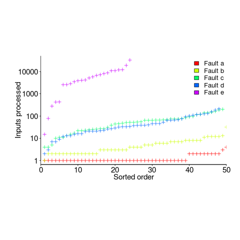
The plot illustrates that some coding mistakes are more likely to produce a fault experience than others (because they are more likely to interact with input values in a way that generates a fault experience), and it also shows how the number of inputs values processed before a particular fault is experienced varies between coding mistakes.
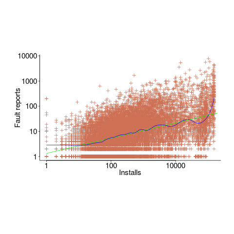
Real-world evidence of the impact of user input on reported faults is provided by the Ultimate Debian Database, which provides information on the number of reported faults and the number of installs for 14,565 packages. The plot below shows how the number of reported faults increases with the number of times a package has been installed; one interpretation is that with more installs there is a wider variety of input values (increasing the likelihood of a fault experience), another is that with more installs there is a larger pool of people available to report a fault experience. Green line is a fitted power law,  , blue line is a fitted loess model.
The source containing a mistake may be executed without a fault being experienced; reasons for this include:
- the input values don’t result in the incorrect code behaving differently from the correct code. For instance, given the made-up incorrect code
if (x < 8)(i.e.,8was typed rather than7), the comparison only produces behavior that differs from the correct code whenxhas the value7, - the input values result in the incorrect code behaving differently than the correct code, but the subsequent path through the code produces the intended external behavior.
Some of the studies that have investigated the program behavior after a mistake has deliberately been introduced include:
- checking the later behavior of a program after modifying the value of a variable in various parts of the source; the results found that some parts of a program were more susceptible to behavioral modification (i.e., runtime behavior changed) than others (i.e., runtime behavior not change),
- checking whether a program compiles and if its runtime behavior is unchanged after random changes to its source code (in this study, short programs written in 10 different languages were used),
- 80% of radiation induced bit-flips have been found to have no externally detectable effect on program behavior.
What are the economic costs and benefits of finding and fixing coding mistakes before shipping vs. waiting to fix just those faults reported by customers?
Checking that a software system exhibits the intended behavior takes time and money, and the organization involved may not be receiving any benefit from its investment until the system starts being used.
In some applications the cost of a fault experience is very high (e.g., lowering the landing gear on a commercial aircraft), and it is cost-effective to make a large investment in gaining a high degree of confidence that the software behaves as expected.
In a changing commercial world software systems can become out of date, or superseded by new products. Given the lifetime of a typical system, it is often cost-effective to ship a system expected to contain many coding mistakes, provided the mistakes are unlikely to be executed by typical customer input in a way that produces a fault experience.
Beta testing provides selected customers with an early version of a new release. The benefit to the software vendor is targeted information about remaining coding mistakes that need to be fixed to reduce customer fault experiences, and the benefit to the customer is checking compatibility of their existing work practices with the new release (also, some people enjoy being able to brag about being a beta tester).
- One study found that source containing a coding mistake was less likely to be changed due to fixing the mistake than changed for other reasons (that had the effect of causing the mistake to disappear),
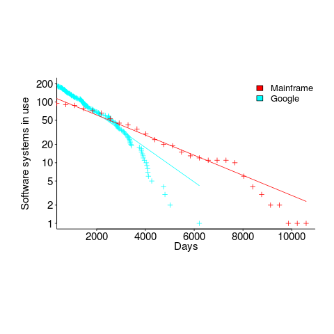
- Software systems don't live forever; systems are replaced or cease being used. The plot below shows the lifetime of 202 Google applications (half-life 2.9 years) and 95 Japanese mainframe applications from the 1990s (half-life 5 years; code+data).
Not only are most coding mistakes not immediately detectable, there may be sound economic reasons for not investing in detecting many of them.
Learning useful stuff from the Reliability chapter of my book
What useful, practical things might professional software developers learn from my evidence-based software engineering book?
Once the book is officially released I need to have good answers to this question (saying: “Well, I decided to collect all the publicly available software engineering data and say something about it”, is not going to motivate people to read the book).
This week I checked the reliability chapter; what useful things did I learn (combined with everything I learned during all the other weeks spent working on this chapter)?
A casual reader skimming the chapter would conclude that little was known about software reliability, and they would be right (I already knew this, but I learned that we know even less than I thought was known), and many researchers continue to dig in unproductive holes.
A reader with some familiarity with reliability research would be surprised to see that some ‘major’ topics are not discussed.
The train wreck that is machine learning has been avoided (not forgetting that the data used is mostly worthless), mutation testing gets mentioned because of some interesting data (the underlying problem is that mutation testing assumes that coding mistakes are local to one line, but in practice coding mistakes often involve multiple lines), and the theory discussions don’t mention non-homogeneous Poisson process as the basis for software fault models (because this process is not capable of solving the questions asked).
What did I learn? My highlights include:
- Anne Choa‘s work on population estimation. The takeaway from this work is that if people want to estimate the number of remaining fault experiences, based on previous experienced faults, then every occurrence (i.e., not just the first) of a fault needs to be counted,
- Phyllis Nagel and Janet Dunham’s top read work on software testing,
- the variability in the numeric percentage that people assign to probability terms (e.g., almost all, likely, unlikely) is much wider than I would have thought,
- the impact of the distribution of input values on fault experiences may be detectable,
- really a lowlight, but there is a lot less publicly available data than I had expected (for the other chapters there was more data than I had expected).
The last decade has seen fuzzing grow to dominate the headlines around software reliability and testing, and provide data for people who write evidence-based books. I don’t have much of a feel for how widely used it is in industry, but it is a very useful tool for reliability researchers.
Readers might have a completely different learning experience from reading the reliability chapter. What useful things did you learn from the reliability chapter?
New users generate more exceptions than existing users (in one dataset)
Application usage data is one of the rarest kinds of public software engineering data.
Even data that might be used to approximate application usage is rare. Server logs might be used as a proxy for browser usage or operating system usage, and number of Debian package downloads as a proxy for usage of packages.
Usage data is an important component of fault prediction models, and the failure to incorporate such data is one reason why existing fault models are almost completely worthless.
The paper Deriving a Usage-Independent Software Quality Metric appeared a few months ago (it’s a bit of a kitchen sink of a paper), and included lots of usage data! As far as I know, this is a first.
The data relates to a mobile based communications App that used Google analytics to log basic usage information, i.e., daily totals of: App usage time, uses by existing users, uses by new users, operating system+version used by the mobile device, and number of exceptions raised by the App.
Working with daily totals means there is likely to be a non-trivial correlation between usage time and number of uses. Given that this is the only public data of its kind, it has to be handled (in my case, ignored for the time being).
I’m expecting to see a relationship between number of exceptions raised and daily usage (the data includes a count of fatal exceptions, which are less common; because lots of data is needed to build a good model, I went with the more common kind). So a’fishing I went.
On most days no exception occurred (zero is the ideal case for the vendor, but I want lots of exception to build a good model). Daily exception counts are likely to be small integers, which suggests a Poisson error model.
It is likely that the same set of exceptions were experienced by many users, rather like the behavior that occurs when fuzzing a program.
Applications often have an initial beta testing period, intended to check that everything works. Lucky for me the beta testing data is included (i.e., more exceptions are likely to occur during beta testing, which get sorted out prior to official release). This is the data I concentrated my modeling.
The model I finally settled on has the form (code+data):

Yes,  had a much bigger impact than
  . This was true for all the models I built using data for all Android/iOS Apps, and the exponent difference was always greater than two.
Why square-root, rather than log? The model fit was much better for square-root; too much better for me to be willing to go with a model which had  as a power-law.
The impact of  varied by several orders of magnitude (which won’t come as a surprise to developers using earlier versions of Android).
There were not nearly as many exceptions once the App became generally available, and there were a lot fewer exceptions for the iOS version.
The outsized impact of new users on exceptions experienced is easily explained by developers failing to check for users doing nonsensical things (which users new to an App are prone to do). Existing users have a better idea of how to drive an App, and tend to do the kind of things that developers expect them to do.
As always, if you know of any interesting software engineering data, please let me know.
Recent Comments