Archive
Distribution of small project completion times
Records of project estimates and actual task times show that round numbers are very common. Various possible reasons have been suggested for why actual times are often reported as a round number. This post analyses the impact of round number reports of actual times on the accuracy of estimates.
The plot below shows the number of tasks having a given reported completion time for 1,525 tasks estimated to take 1-hour (code+data):

Of those 1,525 tasks estimated to take 1-hour, 44% had a reported completion time of 1-hour, 26% took less than 1-hour and 30% took more than 1-hour. The mean is 1.6 hours and the standard deviation 7.1. The spikiness of the distribution of actual times rules out analytical statistical analysis of the distribution.
If a large task is broken down into, say,  smaller tasks, all estimated to take the same amount of time
  , what is the distribution of actual times for the large task?
In the case of just two possible actual times to complete each smaller task, some percentage,  , of tasks are completed in actual time
  , and some percentage,
  , completed in actual time
  (with
(with  ). The probability distribution of the large task time,
 ") , for the two actual times case is:
, for the two actual times case is:
=(matrix{2}{1}{N k})(1-p_{t1})^k {p_{t1}}^{N-k}=(matrix{2}{1}{N k}){p_{t2}}^k (1-p_{t2})^{N-k}")
where:  , and
, and  .
.
The right-most equation is the probability distribution of the Binomial distribution, ") . The possible completion times for the large task start at
. The possible completion times for the large task start at  , followed by time increments of .
When there are three possible actual completion times for each smaller task, the calculation is complicated, and become more complicated with each new possible completion time.
A practical approach is to use Monte Carlo simulation. This involves simulating lots of large tasks containing smaller tasks. A sample of tasks is randomly drawn from the known 1,525 task actual times, and these actual times added to give one possible completion time. Running this process, say, 10,000 times produces what is known as the empirical distribution for the large task completion time.
The plot below shows the empirical distribution  smaller 1-hour tasks. The blue/green points show two peaks, the higher peak is a consequence of the use of round numbers, and the lower peak a consequence of the many non-round numbers. If the total times are rounded to 15 minute times, red points, a smoother distribution with a single peak emerges (code+data):

When a large task involves smaller tasks estimated to take a variety of times, the empirical distribution of the actual time for each estimated time can be combined to give an empirical distribution of the large task (see sum_prob_distrib).
Provided enough information on task completion times is available, this technique works does what it says on the tin.
Why is actual implementation time often reported in whole hours?
Estimates of the time needed to implement a software task are often given in whole hours (i.e., no minutes), with round numbers being preferred. Surprisingly, reported actual implementation times also share this ‘preference’ for whole hours and round numbers (around a third of short task estimates are accurate, so it is to be expected that around a third of actual implementation times will be some number of whole hours, at least for the small percentage of projects that record task implementation time).
Even for accurate estimates, some variation in minutes around the hour boundary is to be expected for the actual implementation time. Why are developers reporting integer hour values for actual time?
The following are some of the possible reasons, two at opposite ends of the spectrum, for developers to log actual time as an integer number of hours:
- Parkinson’s law, i.e., the task was completed earlier and the minutes before the whole hour were filled with other activities,
- striving to complete a task by the end of the hour, much like a marathon runner strives to complete a race on a preselected time boundary,
- performing short housekeeping tasks once the primary task is complete, where management is aware of this overhead accounting.
Is it possible to distinguish between these developer behaviors by analysing many task durations?
My thinking is that all three of these practices occur, with some developers having a preference for following Parkinson’s law, and a few developers always striving to get things done.
Given that Parkinson’s law is 70 years old and well known, there ought to be a trail of research papers analysing a variety of models.
Parkinson specified two ‘laws’. The less well known second law, specifies that the number of bureaucrats in an organization tends to grow, regardless of the amount of work to be done. Governments and large organizations publish employee statistics, and these have been used to check Parkinson’s second law.
With regard to Parkinson’s first law, there are papers whose titles suggest that something more than arm waving is to be found within. Sadly, I have yet to find a non-arm waving paper. Given the extreme difficulty of obtaining data on task durations, this lack of papers is not surprising.
Perhaps our LLM overlords, having been trained on the contents of the Internet, will succeed where traditional search engines have failed. The usual suspects (Grok, ChatGPT, Perplexity and Deepseek) suggested various techniques for fitting models to data, rather than listing existing models.
A new company, Kimi, launched their highly-rated model yesterday, and to try it out I asked: “Discuss mathematical models that analyse the impact of project staff following Parkinson’s law”. The quality of the reply was impressive (my registration has not yet been accepted, so I cannot obtain a link to Kimi’s response). A link to Grok 3’s evaluation of Kimi’s five suggested modelling techniques.
Having spent a some time studying the issues of integer hour actual times, I have not found a way to distinguish between the three possibilities listed above, using estimate/actual time data. Software development involves too many possible changeable activities to be amenable to Taylor’s scientific management approach.
Good luck trying to constrain what developers can do and when they can do it, or requiring excessive logging of activities, just to make it possible to model the development process.
When task time measurements are not reported by developers
Measurements of the time taken to complete a software development task usually rely on the values reported by the person doing the work. People often give round number answers to numeric questions. This rounding has the effect of shifting start/stop/duration times to 5/10/15/20/30/45/60 minute boundaries.
To what extent do developers actually start/stop tasks on round number time boundaries, or aim to work for a particular duration?
The ABB Dev Interaction Data contains 7,812,872 interactions (e.g., clicking an icon) with Visual Studio by 144 professional developers performing an estimated 27,000 tasks over about 28,000 hours. The interaction start/stop times were obtained from the IDE to a 1-second resolution.
Completing a task in Visual Studio involves multiple interactions, and the task start/end times need to be extracted from each developer’s sequence of interactions. Looking at the data, rows containing the File.Exit message look like they are a reliable task-end delimiter (subsequent interactions usually happen many minutes after this message), with the next task for the corresponding developer starting with the next row of data.
Unfortunately, the time between two successive interactions is sometimes so long that it looks as if a task has ended without a File.Exit message being recorded. Plotting the number of occurrences of time-gaps between interactions (in minutes) suggests that it’s probably reasonable to treat anything longer than a 10-minute gap as the end of a task.
The plot below shows the number of tasks having a given duration, based on File.Exit, or using an 11-minute gap between interactions (blue/green) to indicate end-of-task, or a 20-minute gap (red; code+data):

The very prominent spikes in task counts at round numbers, seen in human reported times, are not present. The pattern of behavior is the same for both 11/20-minute gaps. I have no idea why there is a discontinuity at 10 minutes.
A development task is likely to involve multiple VS tasks. Is the duration of multiple VS tasks more likely to sum to a round number than a nonround number? There is no obvious reason why they should.
Is work on a VS task more likely to start/end at a round number time than a nonround number time?
Brief tasks are likely to be performed in the moment, i.e., without regard to clock time. Perhaps developers pay attention to clock time when tasks are expected to take some time.
The plot below shows the number of tasks taking at least 10-minutes that are started at a given number of minutes past the hour (blue/green), with red pluses showing 5-minute intervals (code+data):

No spikes in the count of tasks at round number start times (no spikes in the end times either; code+data).
Why spend time looking for round numbers where they are not expected to occur? Publishing negative results is extremely difficult, and so academics are unlikely to be interested in doing this analysis (not that software engineering researchers have shown any interest in round number usage).
Modelling estimate/actual including uncertainty in the estimate
What is an effective technique for modelling the relationship between the time estimated to implement a task and the actual time taken to implement that task?
A regression model is the obvious approach. However, an important assumption made by the commonly used regression techniques is not met by estimate/actual project data
The commonly used regression techniques involve two kinds of variables: the explanatory variable and the response variable (also known as the independent and dependent variables). For instance, in the equation  ,
,  is the explanatory variable and
  is the response variable.
When fitting a regression model to measurement data, the fitted equation is assumed to have the form such as:  , where
  is uncertainty in the value of , with the valued assumed to have no uncertainty;
  and
and  are constants fitted by the modelling process. The values returned by the model fitting process include an estimate for , as well as estimates for and .
When running an experiment, the values of the explanatory variables(e.g., ) are chosen by the experimenter, with the subject providing the value of the response variable, e.g., .
What does this technical detail have to do with estimation data?
The task estimate/actual values are both provide by the subject (i.e., the developer), there is no experimenter providing one of the values; in fact there is no experiment, these are measurements of things that happened. Both the estimate and actual are response variables, and both contain some amount of uncertainty, and the fitting process needs to take this into account. The appropriate regression technique to use for this case is an errors-in-variables model, which fits the equation +epsilon") , with
, with  being the uncertainty in .
A previous post discussed the surprising behavior that can occur when failing to use errors-in-variables regression for where the data does not contain any explanatory variables, i.e., all the variables contain uncertainty.
The process of fitting an errors-in-variables regression model requires additional input, a value for has to be specified. Taking the example of task estimation, possible uncertainties in the estimate include: misunderstanding of the requirement(s), faded memory of the actual time previously taken by very similar tasks, an inaccurate model of developer skills, and a preference for using round numbers.
What data is available on the uncertainty of individual task estimates? I know of one study where, unknown to them, the individuals estimated the same task twice (in fact, seven people each estimated the same six distinct tasks twice, over a period of three-months). The plot below shows the first/second estimate made by each person for each of the six tasks, with the grey line showing where first==second estimate (code+data):
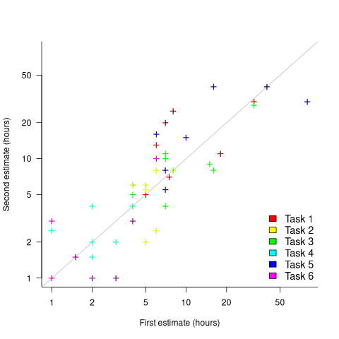
Assuming the estimation uncertainty in this experiment’s data is roughly equal to the estimation uncertainty in other estimation datasets, of tasks taking up to 20 hours, how might it be used to calculate a value for the uncertainty in estimated values?
Two possibilities include:
- Assuming that the uncertainty in both the first and second estimates is equal, a model can be fitted using Deming regression (which treats both variables as having the same uncertainty), and the residual standard error of this model used as the value of . This value for a fitted multiplicative model is 0.6 (code+data),
- using the mean of the relative errors,
}/Est_1") ; its value is 0.55.
; its value is 0.55.
How different are the models built using linear regression and errors-in-variables regression, for small task estimates?
A basic linear regression model fitted to the SiP estimation dataset is:  .
.
Updating this model, using SIMEX, to take into uncertainty in the value of  gives, for an uncertainty error of 0.55:
  , and for an uncertainty error of 0.60:
  . The coefficients for the two models are essentially the same (code+data).
The exponent value is the noticeable difference between the linear regression and errors-in-variables regression models. Adding the assumed amount of uncertainty (based on data from one experiment) to the estimated value leads to a model where estimate/actual are very close to having a linear relationship.
Is this errors-in-variables model any closer to reality than the linear regression model? The model shows that the estimate/actual relationship is closer to linear than was previously thought. Until more data becomes available, we won’t know how close this relationship actually is.
The people who made the estimates in the SiP data also performed the work that took the recorded actual time. Assigning a task to a different person could produce both a different estimate and a different actual, but these possible values are unknown. On a larger scale, different companies bidding on the same contract specify different amounts and have different implementations times; data showing these differences.
A surprising retrospective task estimation dataset
When estimating the time needed to implement a task, the time previously needed to implement similar tasks provides useful guidance. The implementation time for these previous tasks may itself be estimated, because the actual time was not measured or this information is currently unavailable.
How accurate are developer time estimates of previously completed tasks?
I am not aware of any software related dataset of estimates of previously completed tasks (it’s hard enough finding datasets containing information on the actual implementation time). However, I recently found the paper Dynamics of retrospective timing: A big data approach by Balcı, Ünübol, Grondin, Sayar, van Wassenhove, and Wittmann. The data analysed comes from a survey questionnaire, where 24,494 people estimated the how much time they had spent answering the questions, along with recording the current time at the start/end of the questionnaire. The supplementary data is in MATLAB format, and is also available as a csv file in the Blursday database (i.e., RT_Datasets).
Some of the behavior patterns seen in software engineering estimates appear to be general human characteristics, e.g., use of round numbers. An analysis of the estimation performance of a wide sample of the general population could help separate out characteristics that are specific to software engineering and those that apply to the general population.
The following table shows the percentage of answers giving a particular Estimate and Actual time, in minutes. Over 60% of the estimates are round numbers. Actual times are likely to be round numbers because people often give a round number when asked the time (code+data):
   Minutes    Estimate    Actual
     20          18%       8.5%
     15          15%       5.3%
     30          12%       7.6%
     25          10%       6.2%
10 7.7% 2.1% |
I was surprised to see that the authors had fitted a regression model with the Actual time as the explanatory variable and the Estimate as the response variable. The estimation models I have fitted always have the roles of these two variables reversed. More of this role reversal difference below.
The equation fitted to the data by the authors is (they use the term Elapsed, for consistency with other blog articles I continue to use Actual; code+data):

This equation says that, on average, for shorter Actual times the Estimate is higher than the Actual, while for longer Actual times the average Estimate is lower.
Switching the roles of the variables, I expected to see a fitted model whose coefficients are somewhat similar to the algebraically transformed version of this equation, i.e.,  . At the very least, I expected the exponent to be greater than one.
Surprisingly, the equation fitted with the variables roles reversed is very similar, i.e., the equations are the opposite of each other:

This equation says that, on average, for shorter Estimate times the Actual time is higher than the Estimate, while for longer Estimate times the average Actual is lower, i.e., the opposite behavior specifie dby the earlier equation.
I spent some time trying to understand how it was possible for data to be fitted such that (x ~ y) == (y ~ x), even posting a question to Cross Validated. I might, in a future post, discuss the statistical issues behind this behavior.
So why did the authors of this paper treat Actual as an explanatory variable?
After a flurry of emails with the lead author, Fuat Balcı (who was very responsive to my questions), where we both doubled checked the code/data and what we thought was going on, Fuat answered that (quoted with permission):
“The objective duration is the elapsed time (noted by the experimenter based on a clock reading), and the estimate is the participant’s response. According to the psychophysical approach the mapping between objective and subjective time can be defined by regressing the subjective estimates of the participants on the objective duration noted by the experimenter. Thus, if your research question is how human’s retrospective experience of time changes with the duration of events (e.g., biases in time judgments), the y-axis should be the participant’s response and the x-axis should be the actual duration.”
This approach has a logic to it, and is consistent with the regression modelling done by other researchers who study retrospective time estimation.
So which modelling approach is correct, and are people overestimating or underestimating shorter actual time durations?
Going back to basics, the structure of this experiment does not produce data that meets one of the requirements of the statistical technique we are both using (ordinary least squares) to fit a regression model. To understand why ordinary least squares, OLS, is not applicable to this data, it’s necessary to delve into a technical detail about the mathematics of what OLS does.
The equation actually fitted by OLS is:  , where is an error term (i.e., ‘noise’ caused by all the effects other than ). The value of is assumed to be exact, i.e., not contain any ‘noise’.
Usually, in a retrospective time estimation experiment, subjects hear, for instance, a sound whose duration is decided in advance by the experimenter; subjects estimate how long each sound lasted. In this experimental format, it makes sense for the Actual time to appear on the right-hand-side as an explanatory variable and for the Estimate response variable on the left-hand-side.
However, for the questionnaire timing data, both the Estimate and Actual time are decided by the person giving the answers. There is no experimenter controlling one of the values. Both the Estimate and Actual values contain ‘noise’. For instance, on a different day a person may have taken more/less time to actually answer the questionnaire, or provided a different estimate of the time taken.
The correct regression fitting technique to use is errors-in-variables. An errors-in-variables regression fits the equation:  + epsilon") , where:
, where:  is the true value of and is its associated error. A selection of packages are available for fitting a variety of errors-in-variables models.
I regularly see OLS used in software engineering papers (including mine) where errors-in-variables is the technically correct technique to use. Researchers are either unaware of the error issues or assuming that the difference is not important. The few times I have fitted an errors-in-variables model, the fitted coefficients have not been much different from those fitted by an OLS model; for this dataset the coefficient difference is obviously important.
The complication with building an errors-in-variables model is that values need to be specified for the error terms and . With OLS the value of is produced as part of the fitting process.
How might the required error values be calculated?
If some subjects round reported start/stop times, there may not be any variation in reported Actual time, or it may jump around in 5-minute increments depending on the position of the minute hand on the clock.
Learning researchers have run experiments where each subject performs the same task multiple times. Performance improves with practice, which makes it difficult to calculate the likely variability in the first-time performance. If we assume that performance is skill based, the standard deviation of all the subjects completing within a given timeframe could be used to calculate an error term.
With 60% of Estimates being round numbers, there might not be any variation for many people, or perhaps the answer given will change to a different round number. There is Estimate data for different, future tasks, and a small amount of data for the same future tasks. There is data from many retrospective studies using very short time intervals (e.g., tens of seconds), which might be applicable.
We could simply assume that the same amount of error is present in each variable. Deming regression is an errors-in-variables technique that supports this approach, and does not require any error values to be specified. The following equations have been fitted using Deming regression (code+data):

and

While these two equations are consistent with each other, we don’t know if the assumption of equal errors in both variables is realistic.
What next?
Hopefully it will be possible to work out reasonable error values for the Actual/Estimate times. Fitting a model using these values will tell us wether any over/underestimating is occurring, and the associated span of time durations.
I also need to revisit the analysis of software task estimation times.
Rounding in reported task implementation time
There is lots of evidence that people often pick a round number when estimating the time needed to implement a task. Parkinson’s law suggests that reported actual implementation time will often also be a round number, e.g., report 30 minutes for a task that actually took 28 minutes.
If a task is estimated to take 1-hour, what is the distribution of reported implementations times? The analysis in this article uses the SiP task dataset, and similar patterns occur in other datasets.
The plot below shows the number of tasks having a given reported implementation time, for tasks estimated to take 1-hour, with main peaks labelled in red (reported times rounded to one decimal place and quarter hours; code+data):
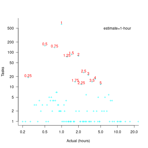
With 1-hour estimates, there is limited scope for a wide range of actual times (at least for times less than estimates). The labelled peaks contain 89% of 1-hour estimate tasks (1,525 tasks, 21% less than estimate, 44% equal estimate, 24% greater than estimate).
Tasks with larger estimated times are likely to take longer, creating more possible rounding peaks in the implementation time distribution. The plot below shows the number of tasks having a given reported implementation time, for tasks estimated to take 7-hour (i.e., 1-day), with main peaks labelled in red (reported times rounded to one decimal place and quarter hours; code+data):
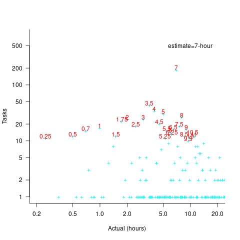
As expected, there are more peaks and implementation times are distributed over a larger range of values.
These plots suggest that many actual times are being rounded to 15-minute intervals. The plot below is based on the minute portion of the reported time (i.e., the hour part is ignored), and shows the fraction of tasks, for estimates of 1, 2, 3, 5, 7, and 14 hours, whose minute component of reported time has a given value (code+data):

For estimates of a few hours, around 90% of reported task time is on a 15-minute mark, while for 7- and 14-hour tasks the percentage drops to 80%.
If staff are manually entering task finish times, then some degree of rounding is to be expected. When the finish time is indirectly calculated, based on the submission of a completed form, there will be some fuzziness to the rounding number process.
Actual implementation times are often round numbers
To what extent do developers consciously influence the time taken to actually complete a task?
If the time estimated to complete a task is rather generous, a developer has the opportunity to follow Parkinson’s law (i.e., “work expands so as to fill the time available for its completion”), or if the time is slightly less than appears to be required, they might work harder to finish within the estimated time (like some marathon runners have a target time)?
The use of round numbers are a prominent pattern seen in task estimation times.
If round numbers appeared more often in the actual task completion time than would be expected by chance, it would suggest that developers are sometimes working to a target time. The following plot shows the number of tasks taking a given amount of actual time to complete, for project 615 in the CESAW dataset (similar patterns are present in the actual times of other projects; code+data):
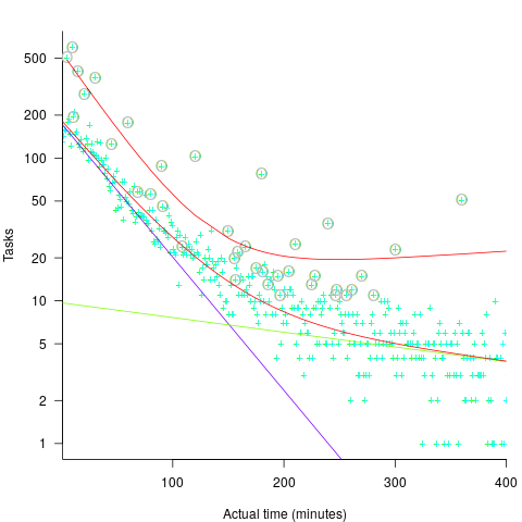
The red lines are a fitted bi-exponential distribution to the ‘spike’ (i.e., round numbers, circled in grey) and non-spike points (spikes automatically selected, see code for details), green and purple lines are the two components of the non-spike fit.
Tasks are not always started and completed in one continuous work session, work may be spread over multiple work sessions; the CESAW data includes the start/end time of every work session associated with each task (85% of tasks involve more than one work session, for project 615). The following plots are based on work sessions, rather than tasks, for tasks worked on over two (left) and three (right) sessions; colored lines denote session ordering within a task (code+data):
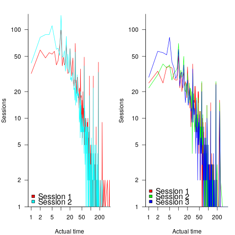
Shorter sessions dominate for the last session of task implementation, and spikes in the counts indicate the use of round numbers in all session positions (e.g., 180 minutes, which may be half a day).
Perhaps round number work session times are a consequence of developers using round number wall-clock times to start and end work sessions. The plot below shows (left) the number of work sessions starting at a given number of minutes past the hour, and (right) the number of work sessions ending at a given number of minutes past the hour; both for project 615 (code+data):
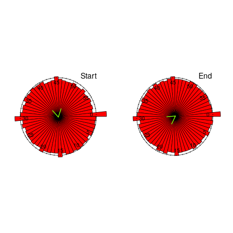
The arrow (green) shows the direction of the mean, and the almost invisible interior line shows that the length of the mean is almost zero. The five-minute points have slightly more session starts/ends than the surrounding minute values, but are more like bumps than spikes. The start of the hour, and 30-minutes, have prominent spikes, which might be caused by the start/end of the working day, and start/end of the lunch break.
Five-minutes is a convenient small rounding interval to either expand implementation time, or to target as a completion time. The following plot shows, for each of the 47 individuals working on project 615, the number of actual session times and the number exactly divisible by five. The green line shows the case where every actual is divisible by five, the purple line where 20% are divisible by five (expected for unbiased timing), the dashed purple lines show one standard deviation, the blue/green line is a fitted regression model ( ) (code+data):
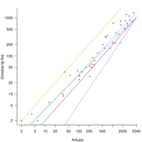
It appears that on average, five-minute session times occur twice as often as expected by chance; two individuals round all their actual session times (ok, it’s not that unlikely for the person with just two sessions).
Does it matter that some developers have a preference for using round numbers when recording time worked?
The use of round numbers in the recording of actual work sessions will inflate the total actual time for most tasks (because most tasks involve more than one session, and assuming that most rounding is not caused by developers striving to meet a target). The amount of error introduced is probably a lot less than the time variability caused by other implementation factors (I have yet to do the calculation).
I see the use of round numbers as a means of unpicking developer work habits.
Given the difficulty of getting developers to record anything, requiring them to record to minute-level accuracy appears at best optimistic. Would you work for a manager that required this level of effort detail (I know there is existing practice in other kinds of jobs)?
Recent Comments