Archive
Learning useful stuff from the Projects chapter of my book
What useful, practical things might professional software developers learn from the Projects chapter in my evidence-based software engineering book?
This week I checked the projects chapter; what useful things did I learn (combined with everything I learned during all the other weeks spent working on this chapter)?
There turned out to be around three to four times more data publicly available than I had first thought. This is good, but there is a trap for the unweary. For many topics there is one data set, and that one data set may not be representative. What is needed is a selection of data from various sources, all relating to a given topic.
Some data is better than no data, provided small data sets are treated with caution.
Estimation is a popular research topic: how long will a project take and how much will it cost.
After reading all the papers I learned that existing estimation models are even more unreliable than I had thought, and what is more, there are plenty of published benchmarks showing how unreliable the models really are (these papers never seem to get cited).
Models that include lines of code in the estimation process (i.e., the majority of models) need a good estimate of the likely number of lines in the final software system. One issue that nobody had considered was the impact of developer variability on the number of lines written to implement the same functionality, which turns out to be large. Oops.
Machine learning has infested effort estimation research. What the machine learning models actually do is estimate adjustment, i.e., they do not create their own estimate but adjust one passed in as input to the model. Most estimation data sets are tiny, and only contain a few different variables; unless the estimate is included in the training phase, the generated model produces laughable results. Oops.
The good news is that there appear to be lots of recurring patterns in the project data. This is good news because recurring patterns are something to be explained by a theory of software project development (apparent randomness is bad news, from the perspective of coming up with a model of what is going on). I think we are still a long way from having workable theories, but seeing patterns is a good sign that one or more theories will be possible.
I think that the main takeaway from this chapter is that software often has a short lifetime. People in industry probably have a vague feeling that this is true, from experience with short-lived projects. It is not cost effective to approach commercial software development from the perspective that the code will live a long time; some code does live a long time, but most dies young. I see the implications of this reality being a major source of contention with those in academia who have spent too long babbling away in front of teenagers (teaching the creation of idealized software that lives on forever), and little or no time building software systems.
A lot of software is written by teams of people, however, there is not a lot of data available on teams (software or otherwise). Given the difficulty of hiring developers, companies have to make do with what they have, so a theory of software teams might not be that useful in practice.
Readers might have a completely different learning experience from reading the projects chapter. What useful things did you learn from the projects chapter?
Learning useful stuff from the Reliability chapter of my book
What useful, practical things might professional software developers learn from my evidence-based software engineering book?
Once the book is officially released I need to have good answers to this question (saying: “Well, I decided to collect all the publicly available software engineering data and say something about it”, is not going to motivate people to read the book).
This week I checked the reliability chapter; what useful things did I learn (combined with everything I learned during all the other weeks spent working on this chapter)?
A casual reader skimming the chapter would conclude that little was known about software reliability, and they would be right (I already knew this, but I learned that we know even less than I thought was known), and many researchers continue to dig in unproductive holes.
A reader with some familiarity with reliability research would be surprised to see that some ‘major’ topics are not discussed.
The train wreck that is machine learning has been avoided (not forgetting that the data used is mostly worthless), mutation testing gets mentioned because of some interesting data (the underlying problem is that mutation testing assumes that coding mistakes are local to one line, but in practice coding mistakes often involve multiple lines), and the theory discussions don’t mention non-homogeneous Poisson process as the basis for software fault models (because this process is not capable of solving the questions asked).
What did I learn? My highlights include:
- Anne Choa‘s work on population estimation. The takeaway from this work is that if people want to estimate the number of remaining fault experiences, based on previous experienced faults, then every occurrence (i.e., not just the first) of a fault needs to be counted,
- Phyllis Nagel and Janet Dunham’s top read work on software testing,
- the variability in the numeric percentage that people assign to probability terms (e.g., almost all, likely, unlikely) is much wider than I would have thought,
- the impact of the distribution of input values on fault experiences may be detectable,
- really a lowlight, but there is a lot less publicly available data than I had expected (for the other chapters there was more data than I had expected).
The last decade has seen fuzzing grow to dominate the headlines around software reliability and testing, and provide data for people who write evidence-based books. I don’t have much of a feel for how widely used it is in industry, but it is a very useful tool for reliability researchers.
Readers might have a completely different learning experience from reading the reliability chapter. What useful things did you learn from the reliability chapter?
Impact of function size on number of reported faults
Are longer functions more likely to contain more coding mistakes than shorter functions?
Well, yes. Longer functions contain more code, and the more code developers write the more mistakes they are likely to make.
But wait, the evidence shows that most reported faults occur in short functions.
This is true, at least in Java. It is also true that most of a Java program’s code appears in short methods (in C 50% of the code is contained in functions containing 114 or fewer lines, while in Java 50% of code is contained in methods containing 4 or fewer lines). It is to be expected that most reported faults appear in short functions. The plot below shows, left: the percentage of code contained in functions/methods containing a given number of lines, and right: the cumulative percentage of lines contained in functions/methods containing less than a given number of lines (code+data):

Does percentage of program source really explain all those reported faults in short methods/functions? Or are shorter functions more likely to contain more coding mistakes per line of code, than longer functions?
Reported faults per line of code is often referred to as: defect density.
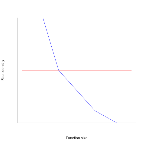
If defect density was independent of function length, the plot of reported faults against function length (in lines of code) would be horizontal; red line below. If every function contained the same number of reported faults, the plotted line would have the form of the blue line below.
Two things need to occur for a fault to be experienced. A mistake has to appear in the code, and the code has to be executed with the ‘right’ input values.
Code that is never executed will never result in any fault reports.
In a function containing 100 lines of executable source code, say, 30 lines are rarely executed, they will not contribute as much to the final total number of reported faults as the other 70 lines.
How does the average percentage of executed LOC, in a function, vary with its length? I have been rummaging around looking for data to help answer this question, but so far without any luck (the llvm code coverage report is over all tests, rather than per test case). Pointers to such data very welcome.
Statement execution is controlled by if-statements, and around 17% of C source statements are if-statements. For functions containing between 1 and 10 executable statements, the percentage that don’t contain an if-statement is expected to be, respectively: 83, 69, 57, 47, 39, 33, 27, 23, 19, 16. Statements contained in shorter functions are more likely to be executed, providing more opportunities for any mistakes they contain to be triggered, generating a fault experience.
Longer functions contain more dependencies between the statements within the body, than shorter functions (I don’t have any data showing how much more). Dependencies create opportunities for making mistakes (there is data showing dependencies between files and classes is a source of mistakes).
The previous analysis makes a large assumption, that the mistake generating a fault experience is contained in one function. This is true for 70% of reported faults (in AspectJ).
What is the distribution of reported faults against function/method size? I don’t have this data (pointers to such data very welcome).
The plot below shows number of reported faults in C++ classes (not methods) containing a given number of lines (from a paper by Koru, Eman and Mathew; code+data):
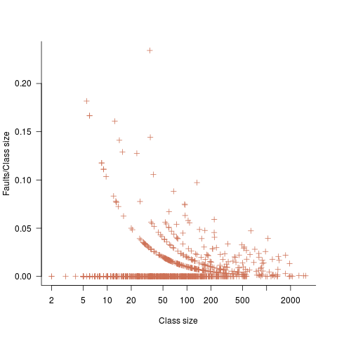
It’s tempting to think that those three curved lines are each classes containing the same number of methods.
What is the conclusion? There is one good reason why shorter functions should have more reported faults, and another good’ish reason why longer functions should have more reported faults. Perhaps length is not important. We need more data before an answer is possible.
The aims of software engineering research
Physics researchers aim to explain the workings of the universe (technically they build models whose behavior mimics that of the universe we can measure), biologists the workings of biological systems, and psychologists the working of the human mind.
What are researchers in software engineering aiming to do?
Talking to academics, the answer is that they aim to do research that can be published in a high impact journal.
What do those involved in commercial software development think software engineering researchers should be aiming to achieve?
Most of the commercial developers I have asked have never thought about the subject; hardly surprising, they have plenty of other issues to think about.
Those who pay for software, rather than create it, want it to be cheaper and delivered faster.
Vendors are under some pressure to reduce costs and deliver sooner. But since its inception, software has been a sellers market, which means the customer pressure does not have the impact it has in other industries.
The very large organizations who pay lots of money for software for their own use (e.g., the U.S. Department of Defence) recognise that research into software production may well save them lots of money, and at one time interesting things were being discovered, but then funding got rerouted to people with an aversion to actual software engineering, i.e., academics.
Cheaper and faster will always be of interest, and will start to become a hot topic in software engineering research once software starts to becoming a buyers market.
Maintaining existing systems continues its growth to dominating what nearly every software developer does. Dependencies on the rest of the software world (e.g., libraries and compilers) is starting to consume a large percentage of maintenance costs. Managers want to know which packages are likely to have a long and stable lifetime, and which are likely to be short-lived. An understanding of the evolution of software ecosystems is a pressing need. This is really cheaper and faster over the long term.
Cheaper and faster (short term for development, long term for maintenance) covers everything.
It’s tempting to list personnel selection, i.e., who is likely to make the best software developer. But why should the process of selecting software developers be any different from the processes used to select people to become doctors, lawyers and other professions? I’m sure that those involved in the various professions would like a magic wand that points to the appropriate people (for some definition of appropriate), this magic wand is no more likely to exist for software developers than any other profession.
What do you think the aims of software engineering research should be?
Time-to-fix when mistake discovered in a later project phase
Traditionally the management of software development projects divides them into phases, e.g., requirements, design, coding and testing. A mistake introduced in one phase may not be detected until a later phase. There is long-standing folklore that earlier mistakes detected in later phases are much much more costly to fix persists, despite the original source of this folklore being resoundingly debunked. Fixing a mistake later is likely to a bit more costly, but how much more costly? A lack of data prevents reliable analysis; this question also suffers from different projects having different cost-to-fix profiles.
This post addresses the time-to-fix question (cost involves all the resources needed to perform the fix). Does it take longer to correct mistakes when they are detected in phases that come after the one in which they were made?
The data comes from the paper: Composing Effective Software Security Assurance Workflows. The 35,367 (yes, thirty-five thousand) logged fixes, from 39 projects drawn from three organizations, contains information on: phases in which the mistake was made and fixed, time taken, person ID, project ID, date/time, plus other stuff 🙂
Every project has its own characteristics that affect time-to-fix. Project 615, avionics software developed by organization A, has the most fixes (7,503) and is analysed here.
Avionics software is safety critical, and each major phase included its own review and inspection. The major phases include: requirements gathering, requirements analysis, high level design, design, coding, and testing. When counting the number of phases between introduction/fix, should review and inspection each count as a phase?
The primary reason for doing a review and inspection is to check the correctness (i.e., lack of mistakes) in the corresponding phase. If there is a time-to-fix penalty for mistakes found in these symbiotic-phases, I suspect it will be different from the time-to-fix penalty between major phases (which for simplicity, I’m assuming is major-phase independent).
The time-to-fix has a resolution of 1-minute, and some fix times are listed as taking a minute; 72% of fixes are recorded as taking less than 10-minutes. What kind of mistakes require less than 10-minutes to fix? Typos and other minutiae.
The plot below shows time-to-fix for mistakes having a given ‘distance’ between introduction/fix phase, for fixes taking at least 1, 5 and 10-minutes (code+data):
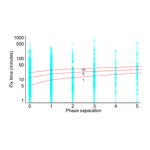
There is a huge variation in time-to-fix, and the regression lines (which have the form:  ) explains just 6% of the variance in the data, i.e., there is a small increase with phase separation, but it is almost down in the noise.
All but one of the 38 people who worked on the project made multiple fixes (30 made more than 20 fixes), and may have got faster with practice. Adding the number of previous fixes by people making more than 20 fixes to the model gives:  , and improves the model by less than 1-percent.
Fixing mistakes is a human activity, and individual performance often has a big impact on fitted models. Adding person ID to the model as a multiplication factor: i.e.,  , improves the variance explained to 14% (better than a poke in the eye, just). The fitted value of
  varies between 0.66 and 1.4 (factor of two, human variation).
The answer to the time-to-fix question posed earlier (for project 615), is that it does take slightly longer to fix a mistake detected in phases occurring after the one in which the mistake was introduced. The phase difference is tiny, with differences in human performance having a bigger impact.
Quality control in a zero cost of replication business
When a new manufacturing material becomes available, its use is often integrated with existing techniques, e.g., using scientific management techniques for software production.
Customers want reliable products, and companies that sell unreliable products don’t make money (and may even lose lots of money).
Quality assurance of manufactured products is a huge subject, and lots of techniques have been developed.
Needless to say, quality assurance techniques applied to the production of hardware are often touted (and sometimes applied) as the solution for improving the quality of software products (whatever quality is currently being defined as).
There is a fundamental difference between the production of hardware and software:
- Hardware is designed, a prototype made and this prototype refined until it is ready to go into production. Hardware production involves duplicating an existing product. The purpose of quality control for hardware production is ensuring that the created copies are close enough to identical to the original that they can be profitably sold. Industrial design has to take into account the practicalities of mass production, e.g., can this device be made at a low enough cost.
- Software involves the same design, prototype, refinement steps, in some form or another. However, the final product can be perfectly replicated at almost zero cost, e.g., downloadable file(s), burn a DVD, etc.
Software production is a once-off process, and applying techniques designed to ensure the consistency of a repetitive process don’t sound like a good idea. Software production is not at all like mass production (the build process comes closest to this form of production).
Sometimes people claim that software development does involve repetition, in that a tiny percentage of the possible source code constructs are used most of the time. The same is also true of human communications, in that a few words are used most of the time. Does the frequent use of a small number of words make speaking/writing a repetitive process in the way that manufacturing identical widgets is repetitive?
The virtually zero cost of replication (and distribution, via the internet, for many companies) does more than remove a major phase of the traditional manufacturing process. Zero cost of replication has a huge impact on the economics of quality control (assuming high quality is considered to be equivalent to high reliability, as measured by number of faults experienced by customers). In many markets it is commercially viable to ship software products that are believed to contain many mistakes, because the cost of fixing them is so very low; unlike the cost of hardware, which is non-trivial and involves shipping costs (if only for a replacement).
Zero defects is not an economically viable mantra for many software companies. When companies employ people to build the same set of items, day in day out, there is economic sense in having them meet together (e.g., quality circles) to discuss saving the company money, by reducing production defects.
Many software products have a short lifespan, source code has a brief and lonely existence, and many development projects are never shipped to paying customers.
In software development companies it makes economic sense for quality circles to discuss the minimum number of known problems they need to fix, before shipping a product.
Extreme value theory in software engineering
As its name suggests, extreme value theory deals with extreme deviations from the average, e.g., how often will rainfall be heavy enough to cause a river to overflow its banks.
The initial list of statistical topics I thought ought to be covered in my evidence-based software engineering book included extreme value theory. At the time, and even today, there were/are no books covering “Statistics for software engineering”, so I had no prior work to guide my selection of topics. I was keen to cover all the important topics, had heard of it in several (non-software) contexts and jumped to the conclusion that it must be applicable to software engineering.
Years pass: the draft accumulate a wide variety of analysis techniques applied to software engineering data, but, no use of extreme value theory.
Something else does not happen: I don’t find any ‘Using extreme value theory to analyse data’ books. Yes, there are some really heavy-duty maths books available, but nothing of a practical persuasion.
The book’s Extreme value section becomes a subsection, then a subsubsection, and ended up inside a comment (I cannot bring myself to delete it).
It appears that extreme value theory is more talked about than used. I can understand why. Extreme events are newsworthy; rivers that don’t overflow their banks are not news.
Just over a month ago a discussion cropped up on the UK’s C++ standards’ panel mailing list: was email traffic down because of COVID-19? The panel’s convenor, Roger Orr, posted some data on monthly volumes. Oh, data 🙂
Monthly data is a bit too granular for detailed analysis over relatively short periods. After some poking around Roger was able to send me the date&time of every post to the WG21‘s Core and Lib reflectors, since February 2016 (there have been various changes of hosts and configurations over the years, and date of posts since 2016 was straightforward to obtain).
During our email exchanges, Roger had mentioned that every now and again a huge discussion thread comes out of nowhere. Woah, sounds like WG21 could do with some extreme value theory. How often are huge discussion threads likely to occur, and how huge is a once in 10-years thread that they might have to deal with?
There are two techniques for analysing the distribution of extreme values present in a sample (both based around the generalized extreme value distribution):
- Generalized Extreme Value (GEV) uses block maxima, e.g., maximum number of daily emails sent in each month,
- Generalized Pareto (GP) uses peak over threshold: pick a threshold and extract day values for when more than this threshold number of emails was sent.
The plots below show the maximum number of monthly emails that are expected to occur (y-axis) within a given number of months (x-axis), for WG21’s Core and Lib email lists. The circles are actual occurrences, and dashed lines 95% confidence intervals; GEV was used for these fits (code+data):
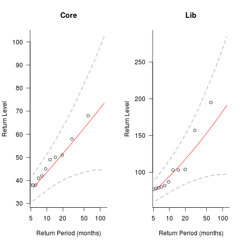
The 10-year return value for Core is around a daily maximum of 70 +-30, and closer to 200 +-100 for Lib.
The model used is very simplistic, and fails to take into account the growth in members joining these lists and traffic lost when a new mailing list is created for a new committee subgroup.
If any readers have suggests for uses of extreme value theory in software engineering, please let me know.
Postlude. This discussion has reordered events. My original interest in the mailing list data was the desire to find some evidence for the hypothesis that the volume of email increased as the date of the next WG21 meeting approached. For both Core and Lib, the volume actually decreases slightly as the date of the next meeting approaches; see code for details. Also, the volume of email at the weekend is around 60% lower than during weekdays.
Scientific management of software production
When Frederick Taylor investigated the performance of workers in various industries, at the start of the 1900’s, he found that workers organise their work to suit themselves; workers were capable of producing significantly more than they routinely produced. This was hardly news. What made Taylor’s work different was that having discovered the huge difference between actual worker output and what he calculated could be achieved in practice, he was able to change work practices to achieve close to what he had calculated to be possible. Changing work practices took several years, and the workers did everything they could to resist it (Taylor’s The principles of scientific management is an honest and revealing account of his struggles).
Significantly increasing worker output pushed company profits through the roof, and managers everywhere wanted a piece of the action; scientific management took off. Note: scientific management is not a science of work, it is a science of the management of other people’s work.
The scientific management approach has been successfully applied to production where most of the work can be reduced to purely manual activities (i.e., requiring little thinking by those who performed them). The essence of the approach is to break down tasks into the smallest number of component parts, to simplify these components so they can be performed by less skilled workers, and to rearrange tasks in a way that gives management control over the production process. Deskilling tasks increases the size of the pool of potential workers, decreasing labor costs and increasing the interchangeability of workers.
Given the almost universal use of this management technique, it is to be expected that managers will attempt to apply it to the production of software. The software factory was tried, but did not take-off. The use of chief programmer teams had its origins in the scarcity of skilled staff; the idea is that somebody who knows what they were doing divides up the work into chunks that can be implemented by less skilled staff. This approach is essentially the early stages of scientific management, but it did not gain traction (see “Programmers and Managers: The Routinization of Computer Programming in the United States” by Kraft).
The production of software is different in that once the first copy has been created, the cost of reproduction is virtually zero. The human effort invested in creating software systems is primarily cognitive. The division between management and workers is along the lines of what they think about, not between thinking and physical effort.
Software systems can be broken down into simpler components (assuming all the requirements are known), but can the implementation of these components be simplified such that they can be implemented by less skilled developers? The process of simplification is practical when designing a system for repetitive reproduction (e.g., making the same widget again and again), but the first implementation of anything is unlikely to be simple (and only one implementation is needed for software).
If it is not possible to break down the implementation such that most of the work is easy to do, can we at least hire the most productive developers?
How productive are different developers? Programmer productivity has been a hot topic since people started writing software, but almost no effective research has been done.
I have no idea how to measure programmer productivity, but I do have some ideas about how to measure their performance (a high performance programmer can have zero productivity by writing programs, faster than anybody else, that don’t do anything useful, from the client’s perspective).
When the same task is repeatedly performed by different people it is possible to obtain some measure of average/minimum/maximum individual performance.
Task performance improves with practice, and an individual’s initial task performance will depend on their prior experience. Measuring performance based on a single implementation of a task provides some indication of minimum performance. To obtain information on an individual’s maximum performance they need to be measured over multiple performances of the same task (and of course working in a team affects performance).
Should high performance programmers be paid more than low performance programmers (ignoring the issue of productivity)? I am in favour of doing this.
What about productivity payments, e.g., piece work?
This question is a minefield of issues. Manual workers have been repeatedly found to set informal quotas amongst themselves, i.e., setting a maximum on the amount they will produce during a shift (see “Money and Motivation: An Analysis of Incentives in Industry” by William Whyte). Thankfully, I don’t think I will be in a position to have to address this issue anytime soon (i.e., I don’t see a reliable measure of programmer productivity being discovered in the foreseeable future).
Surveys are fake research
For some time now, my default position has been that software engineering surveys, of the questionnaire kind, are fake research (surveys of a particular research field used to be worth reading, but not so often these days; that issues is for another post). Every now and again a non-fake survey paper pops up, but I don’t consider the cost of scanning all the fake stuff to be worth the benefit of finding the rare non-fake survey.
In theory, surveys could be interesting and worth reading about. Some of the things that often go wrong in practice include:
- poorly thought out questions. Questions need to be specific and applicable to the target audience. General questions are good for starting a conversation, but analysis of the answers is a nightmare. Perhaps the questions are non-specific because the researcher is looking for direction: well please don’t inflict your search for direction on the rest of us (a pointless plea in the fling it at the wall to see if it sticks world of academic publishing).
Questions that demonstrate how little the researcher knows about the topic serve no purpose. The purpose of a survey is to provide information of interest to those in the field, not as a means of educating a researcher about what they should already know,
- little effort is invested in contacting a representative sample. Questionnaires tend to be sent to the people that the researcher has easy access to, i.e., a convenience sample. The quality of answers depends on the quality and quantity of those who replied. People who run surveys for a living put a lot of effort into targeting as many of the right people as possible,
- sloppy and unimaginative analysis of the replies. I am so fed up with seeing an extensive analysis of the demographics of those who replied. Tables containing response break-down by age, sex, type of degree (who outside of academia cares about this) create a scientific veneer hiding the lack of any meaningful analysis of the issues that motivated the survey.
Although I have taken part in surveys in the past, these days I recommend that people ignore requests to take part in surveys. Your replies only encourage more fake research.
The aim of this post is to warn readers about the growing use of this form of fake research. I don’t expect anything I say to have any impact on the number of survey papers published.
Effort estimation’s inaccurate past and the way forward
Almost since people started building software systems, effort estimation has been a hot topic for researchers.
Effort estimation models are necessarily driven by the available data (the Putnam model is one of few whose theory is based on more than arm waving). General information about source code can often be obtained (e.g., size in lines of code), and before package software and open source, software with roughly the same functionality was being implemented in lots of organizations.
Estimation models based on source code characteristics proliferated, e.g., COCOMO. What these models overlooked was human variability in implementing the same functionality (a standard deviation that is 25% of the actual size is going to introduce a lot of uncertainty into any effort estimate), along with the more obvious assumption that effort was closely tied to source code characteristics.
The advent of high-tech clueless button pushing machine learning created a resurgence of new effort estimation models; actually they are estimation adjustment models, because they require an initial estimate as one of the input variables. Creating a machine learned model requires a list of estimated/actual values, along with any other available information, to build a mapping function.
The sparseness of the data to learn from (at most a few hundred observations of half-a-dozen measured variables, and usually less) has not prevented a stream of puffed-up publications making all kinds of unfounded claims.
Until a few years ago the available public estimation data did not include any information about who made the estimate. Once estimation data contained the information needed to distinguish the different people making estimates, the uncertainty introduced by human variability was revealed (some consistently underestimating, others consistently overestimating, with 25% difference between two estimators being common, and a factor of two difference between some pairs of estimators).
How much accuracy is it realistic to expect with effort estimates?
At the moment we don’t have enough information on the software development process to be able to create a realistic model; without a realistic model of the development process, it’s a waste of time complaining about the availability of information to feed into a model.
I think a project simulation model is the only technique capable of creating a good enough model for use in industry; something like Abdel-Hamid’s tour de force PhD thesis (he also ignores my emails).
We are still in the early stages of finding out the components that need to be fitted together to build a model of software development, e.g., round numbers.
Even if all attempts to build such a model fail, there will be payback from a better understanding of the development process.
Recent Comments