The Shape of Code

It is often said, with some evidence, that 80% of reported faults, for a program, occur in 20% of its code. I think this pattern is a consequence of 20% of the code being executed 80% of the time, while many researchers believe that 20% of the source code has characteristics that result in it containing 80% of the coding mistakes.

The 20% figure is commonly measured as a percentage of methods/functions, rather than a percentage of lines of code.

This post investigates the expected fraction of a program’s methods that remain fault report free, based on two probability models.

Both models assume that coding mistakes are uniformly scattered throughout the code (i.e., every statement has the same probability of containing a mistake) and that the corresponding coding mistake is contained within a single method (the evidence suggests that this is true for 50% of faults).

A simple model is to assume that when a new fault is reported, the probability that the corresponding coding mistake appears in a particular method is proportional to the method’s length, in lines of code, of the method. The evidence shows that the distribution of methods containing a given number of lines, , is well-fitted by a power law (for Java: ).

If reported faults have been fixed in a program containing methods/functions, what is the expected number of methods that have not been modified by the fixing process?

The answer (with help from: mostly Kimi, with occasional help from Deepseek (who don’t have a share chat options), ChatGPT 5, Grok, and some approximations; chat logs) is:

where: is the Riemann zeta function, is the polylogarithm function and for Java.

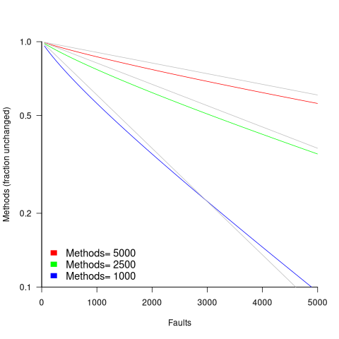
The plot below shows the predicted fraction of unmodified methods against number of faults, for programs of various sizes; the grey lines show the rough approximation: (code+data):

The observed behavior of most reported faults involving a subset of a program’s methods can be modelled using some form of preferential attachment.

One preferential attachment model specifies that the likelihood of a coding mistake appearing in a method is proportional to , where is the number of previously detected coding mistakes in the method.

The estimated number of unmodified methods is now:

where: is the average value of over all faults (if , then for a power law with exponent 2.35).

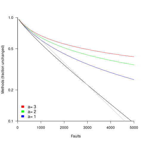
The plot below shows the predicted fraction of unmodified methods against number of faults for a program containing 1,000 methods, for various values of , with the black line showing the fraction of unmodified methods predicted by the simple model above (code+data):

In practice, random selection of the method containing a coding mistake will introduce some fuzziness in the predicted fraction of unmodified methods.

As the number of reported faults grows, the attraction of methods involved in previous reported faults slows the rate at which methods experience their first detected coding mistake.

How realistic are these models?

By focusing on the number of unmodified methods, many complications are avoided.

Both models assume that an unchanging number of methods in a program and that the length of each method is fixed. This assumption holds between each release of a program.

For actively maintained programs, the number of methods in a program changes over time, and the length of some existing methods also changes (if a program were not actively maintained, reported faults would not get fixed).

These models are unlikely to be applicable to programs with short release cycles, where there are few reported faults between releases.

How well do the models’ predictions agree with the data?

At the moment, I am not aware of a dataset containing the appropriate data. Number of faults vs unmodified methods has been added to my list of interesting patterns to notice.

Summary of the derivation of the solutions for the two models.

Simple model

The expected number of unmodified methods, , is:

, where is the length of the longest method, is the number of methods of length , and is the probability that a method of length will be unmodified after fault reports.

The evidence shows that the distribution of methods containing a given number of lines, , is well-fitted by a power law (for Java: ).

Given a program containing methods, the number of methods of length is:

, where for Java.

If is large and , then the sum can be approximated by the Riemann zeta function, , giving:

The probability that a method containing lines will not be modified by a fault report (assuming that fixing the mistake only involves one method) is: , where is the total lines of code in the program, and the probability of this method not being modified after fault reports is approximately:

The expected number of empty boxes is:

The number of lines of code in a program containing methods is:

Finally giving:

where is the polylogarithm function.

This equation is roughly, for the purposes of understanding the effect of each variable:

Preferential attachment model

When a mistake is corrected in a method, the attraction weight of that method increases (alternatively, the attraction weight of the other methods decreases). The probability that a method is not modified after fault reports is now:

where: the average value of over all faults, and is the gamma function.

applying the Stirling/Gamma–ratio rule, i.e., we get:

where the expression is the preferential attachment version of the expression appearing in the simple model derivation. Using this preferential attachment expression in the analysis of the simple model, we get:

I don’t have a rough approximation for this expression.