Archive
When task time measurements are not reported by developers
Measurements of the time taken to complete a software development task usually rely on the values reported by the person doing the work. People often give round number answers to numeric questions. This rounding has the effect of shifting start/stop/duration times to 5/10/15/20/30/45/60 minute boundaries.
To what extent do developers actually start/stop tasks on round number time boundaries, or aim to work for a particular duration?
The ABB Dev Interaction Data contains 7,812,872 interactions (e.g., clicking an icon) with Visual Studio by 144 professional developers performing an estimated 27,000 tasks over about 28,000 hours. The interaction start/stop times were obtained from the IDE to a 1-second resolution.
Completing a task in Visual Studio involves multiple interactions, and the task start/end times need to be extracted from each developer’s sequence of interactions. Looking at the data, rows containing the File.Exit message look like they are a reliable task-end delimiter (subsequent interactions usually happen many minutes after this message), with the next task for the corresponding developer starting with the next row of data.
Unfortunately, the time between two successive interactions is sometimes so long that it looks as if a task has ended without a File.Exit message being recorded. Plotting the number of occurrences of time-gaps between interactions (in minutes) suggests that it’s probably reasonable to treat anything longer than a 10-minute gap as the end of a task.
The plot below shows the number of tasks having a given duration, based on File.Exit, or using an 11-minute gap between interactions (blue/green) to indicate end-of-task, or a 20-minute gap (red; code+data):

The very prominent spikes in task counts at round numbers, seen in human reported times, are not present. The pattern of behavior is the same for both 11/20-minute gaps. I have no idea why there is a discontinuity at 10 minutes.
A development task is likely to involve multiple VS tasks. Is the duration of multiple VS tasks more likely to sum to a round number than a nonround number? There is no obvious reason why they should.
Is work on a VS task more likely to start/end at a round number time than a nonround number time?
Brief tasks are likely to be performed in the moment, i.e., without regard to clock time. Perhaps developers pay attention to clock time when tasks are expected to take some time.
The plot below shows the number of tasks taking at least 10-minutes that are started at a given number of minutes past the hour (blue/green), with red pluses showing 5-minute intervals (code+data):

No spikes in the count of tasks at round number start times (no spikes in the end times either; code+data).
Why spend time looking for round numbers where they are not expected to occur? Publishing negative results is extremely difficult, and so academics are unlikely to be interested in doing this analysis (not that software engineering researchers have shown any interest in round number usage).
Deep dive looking for good enough reliability models
A previous post summarised the main highlights of my trawl through the software reliability research papers/reports/data, which failed to find any good enough models for estimating the reliability of a software system. This post summarises a deep dive into the technical aspects of the research papers.
I am now a lot more confident that better than worst case models for calculating software reliability don’t yet exist (perhaps the problem does not have a solution). By reliability, I mean the likelihood that a fault will be experienced during 1-hour of operation (1-hour is the time interval often used in safety critical standards).
All the papers assume that time to next new fault experience can be effectively modelled using timing information on the previously discovered distinct faults. Timing information might be cpu time, or elapsed time during testing or customer use, or even number of tests. Issues of code coverage and the correspondence between tests and customer usage are rarely mentioned.
Building a model requires making assumptions about the world. Given the data used, all the models assume that there is a relationship connecting the time between successive distinct faults, e,g, the Jelinski-Moranda model assumes that the time between fault experiences has an exponential distribution and that the exponent is the same for all faults. While the Jelinski-Moranda model does not match the behavior seen in the available datasets, it is widely discussed (its simplicity makes it a great example, with the analysis being straightforward and the result easy to explain).
Much of the fault timing data comes from the test process, with the rest coming from customer usage (either cpu or elapsed; like today’s cloud usage, mainframe time usage was often charged). What connection does a model fitted to data on the faults discovered during testing have with faults experienced by customers using the software? Managers want to minimise the cost of testing (one claimed use case for these models is estimating the likelihood of discovering a new fault during testing), and maximising the number of faults found probably has a higher priority than mimicking customer usage.
The early software reliability papers (i.e., the 1970s) invariably proposed a new model and then checked how well it fitted a small dataset.
While the top, must-read paper on software fault analysis was published in 1982, it has mostly remained unknown/ignored (it appeared as a NASA report written by non-academics who did not then promote their work). Perhaps if Nagel and Skrivan’s work had become widely known, today we might have a practical software reliability model.
Reliability research in the 1980s was dominated by theoretical analysis of the previously proposed models and their variants, finding connections between them and building more general models. Ramos’s 2009 PhD thesis contains a great overview of popular (academic) reliability models, their interconnections, and using them to calculate a number.
I did discover some good news. Researchers outside of software engineering have been studying a non-software problem whose characteristics have a direct mapping to software reliability. This non-software problem involves sampling from a population containing subpopulations of varying sizes (warning: heavy-duty maths), e.g., oil companies searching for new oil fields of unknown sizes. It looks, perhaps (the maths is very hard going), as-if the statisticians studying this problem have found some viable solutions. If I’m lucky, I will find a package implementing the technical details, or find a gentle introduction. Perhaps this thread will have a happy ending…
An aside: When quickly deciding whether a research paper is worth reading, if the title or abstract contains a word on my ignore list, the paper is ignored. One consequence of this recent detailed analysis is that the term NHPP has been added to my ignore list for software reliability issues (it has applicability for hardware).
Parkinson’s law, striving to meet a deadline, or happenstance?
How many minutes past the hour was it, when you stopped working on some software related task?
There are sixty minutes in an hour, so if stop times are random, the probability of finishing at any given minute is 1-in-60. If practice (based on the 200k+ time records in the CESAW dataset) the probability of stopping on the hour is 1-in-40, and for stopping on the half-hour is 1-in-48.
Why are developers more likely to stop working on a task, on the hour or half-hour?
Is this a case of Parkinson’s law, or are developers striving to complete a task within a specified time, or are they stopping because a scheduled activity takes priority?
The plot below shows the number of times (y-axis) work on a task stopped on a given minute past the hour (x-axis), for 16 different software projects (project number in blue, with top 10 numbers in red, code+data):
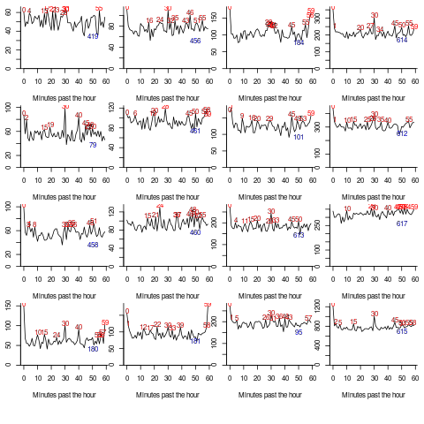
Some projects have peaks at 50, 55, or thereabouts. Perhaps people are stopping because they have a meeting to attend, and a peak is visible because the project had lots of meetings, or no peak was visible because the project had few meetings. Some projects have a peak at 28 or 29, which might be some kind of time synchronization issue.
Is it possible to analyze the distribution of end minutes to reasonably infer developer project behavior, e.g., Parkinson’s law, striving to finish by a given time, or just not watching the clock?
An expected distribution pattern for both Parkinson’s law, and striving to complete, is a sharp decline of work stops after a reference time, e.g., end of an hour (this pattern is present in around ten of the projects plotted). A sharp increase in work stops prior to a reference time could also apply for both behaviors; stopping to switch to other work adds ‘noise’ to the distribution.
The CESAW data is organized by project, not developer, i.e., it does not list everything a developer did during the day. It is possible that end-of-hour work stops are driven by the need to synchronize with non-project activities, i.e., no Parkinson’s law or striving to complete.
In practice, some developers may sometimes follow Parkinson’s law, other times strive to complete, and other times not watch the clock. If models capable of separating out the behaviors were available, they might only be viable at the individual level.
Stop time equals start time plus work duration. If people choose a round number for the amount of work time, there is likely to be some correlation between start/end minutes past the hour. The plot below shows heat maps for start fraction of hour (y-axis) against end fraction of hour (x-axis) for four projects (code+data):
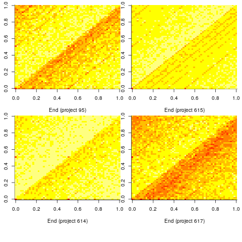
Work durations that are exact multiples of an hour appear along the main diagonal, with zero/zero being the most common start/end pair (at 4% over all projects, with 0.02% expected for random start/end times). Other diagonal lines come from work durations that include a fraction of an hour, e.g., 30-minutes and 20-minutes.
For most work periods, the start minute occurs before the end minute, i.e., the work period does not cross an hour boundary.
What can be learned from this analysis?
The main takeaway is that there is a small bias for work start/end times to occur on the hour or half-hour, and other activities (e.g., meetings) cause ongoing work to be interrupted. Not exactly news.
More interesting ideas and suggestions welcome.
Actual implementation times are often round numbers
To what extent do developers consciously influence the time taken to actually complete a task?
If the time estimated to complete a task is rather generous, a developer has the opportunity to follow Parkinson’s law (i.e., “work expands so as to fill the time available for its completion”), or if the time is slightly less than appears to be required, they might work harder to finish within the estimated time (like some marathon runners have a target time)?
The use of round numbers are a prominent pattern seen in task estimation times.
If round numbers appeared more often in the actual task completion time than would be expected by chance, it would suggest that developers are sometimes working to a target time. The following plot shows the number of tasks taking a given amount of actual time to complete, for project 615 in the CESAW dataset (similar patterns are present in the actual times of other projects; code+data):
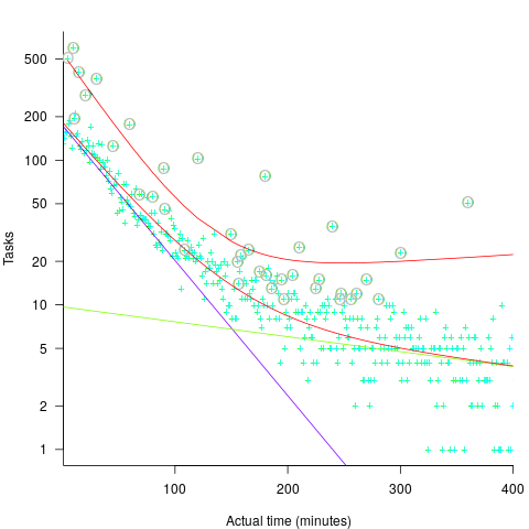
The red lines are a fitted bi-exponential distribution to the ‘spike’ (i.e., round numbers, circled in grey) and non-spike points (spikes automatically selected, see code for details), green and purple lines are the two components of the non-spike fit.
Tasks are not always started and completed in one continuous work session, work may be spread over multiple work sessions; the CESAW data includes the start/end time of every work session associated with each task (85% of tasks involve more than one work session, for project 615). The following plots are based on work sessions, rather than tasks, for tasks worked on over two (left) and three (right) sessions; colored lines denote session ordering within a task (code+data):
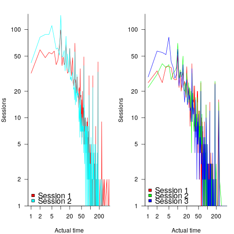
Shorter sessions dominate for the last session of task implementation, and spikes in the counts indicate the use of round numbers in all session positions (e.g., 180 minutes, which may be half a day).
Perhaps round number work session times are a consequence of developers using round number wall-clock times to start and end work sessions. The plot below shows (left) the number of work sessions starting at a given number of minutes past the hour, and (right) the number of work sessions ending at a given number of minutes past the hour; both for project 615 (code+data):
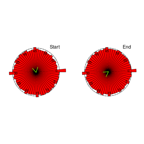
The arrow (green) shows the direction of the mean, and the almost invisible interior line shows that the length of the mean is almost zero. The five-minute points have slightly more session starts/ends than the surrounding minute values, but are more like bumps than spikes. The start of the hour, and 30-minutes, have prominent spikes, which might be caused by the start/end of the working day, and start/end of the lunch break.
Five-minutes is a convenient small rounding interval to either expand implementation time, or to target as a completion time. The following plot shows, for each of the 47 individuals working on project 615, the number of actual session times and the number exactly divisible by five. The green line shows the case where every actual is divisible by five, the purple line where 20% are divisible by five (expected for unbiased timing), the dashed purple lines show one standard deviation, the blue/green line is a fitted regression model ( ) (code+data):
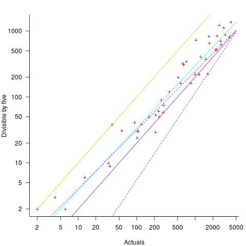
It appears that on average, five-minute session times occur twice as often as expected by chance; two individuals round all their actual session times (ok, it’s not that unlikely for the person with just two sessions).
Does it matter that some developers have a preference for using round numbers when recording time worked?
The use of round numbers in the recording of actual work sessions will inflate the total actual time for most tasks (because most tasks involve more than one session, and assuming that most rounding is not caused by developers striving to meet a target). The amount of error introduced is probably a lot less than the time variability caused by other implementation factors (I have yet to do the calculation).
I see the use of round numbers as a means of unpicking developer work habits.
Given the difficulty of getting developers to record anything, requiring them to record to minute-level accuracy appears at best optimistic. Would you work for a manager that required this level of effort detail (I know there is existing practice in other kinds of jobs)?
Recent Comments