Archive
Impact of developer uncertainty on estimating probabilities
For over 50 years, it has been known that people tend to overestimate the likelihood of uncommon events/items occurring, and underestimate the likelihood of common events/items. This behavior has replicated in many experiments and is sometimes listed as a so-called cognitive bias.
Cognitive bias has become the term used to describe the situation where the human response to a problem (in an experiment) fails to match the response produced by the mathematical model that researchers believe produces the best output for this kind of problem. The possibility that the mathematical models do not reflect the reality of the contexts in which people have to solve the problems (outside of psychology experiments), goes against the grain of the idealised world in which many researchers work.
When models take into account the messiness of the real world, the responses are a closer match to the patterns seen in human responses, without requiring any biases.
The 2014 paper Surprisingly Rational: Probability theory plus noise explains biases in judgment by F. Costello and P. Watts (shorter paper), showed that including noise in a probability estimation model produces behavior that follows the human behavior patterns seen in practice.
If a developer is asked to estimate the probability that a particular event,  , occurs, they may not have all the information needed to make an accurate estimate. They may fail to take into account some s, and incorrectly include other kinds of events as being s. This noise,
  , introduces a pattern into the developer estimate:
*P_E + N*(1-P_E)=(1-2N)*P_E+N")
where:  is the developer’s estimated probability of event occurring,
  is the actual probability of the event, and is the probability that noise produces an incorrect classification of an event as
  or (for simplicity, the impact of noise is assumed to be the same for both cases).
The plot below shows actual event probability against developer estimated probability for various values of , with a red line showing that at  , the developer estimate matches reality (code):

The effect of noise is to increase probability estimates for events whose actually probability is less than 0.5, and to decrease the probability when the actual is greater than 0.5. All estimates move towards 0.5.
What other estimation behaviors does this noise model predict?
If there are two events, say  and
and  , then the noise model (and probability theory) specifies that the following relationship holds:
+P(B) == P(A & B)+P(A delim{|}{B}{})")
where: ") denotes the probability of its argument.
denotes the probability of its argument.
The experimental results show that this relationship does hold, i.e., the noise model is consistent with the experiment results.
This noise model can be used to explain the conjunction fallacy, i.e., Tversky & Kahneman’s famous 1970s “Lindy is a bank teller” experiment.
What predictions does the noise model make about the estimated probability of experiencing  (
( ) occurrences of the event in a sequence of
  assorted events (the previous analysis deals with the case
  )?
)?
An estimation model that takes account of noise gives the equation:

where:  is the developer’s estimated probability of experiencing s in a sequence of length , and
  is the actual probability of there being .
The plot below shows actual event probability against developer estimated probability for various values of , with a red line showing that at , the developer estimate matches reality (code):

This predicted behavior, which is the opposite of the case where , follows the same pattern seen in experiments, i.e., actual probabilities less than 0.5 are decreased (towards zero), while actual probabilities greater than 0.5 are increased (towards one).
There have been replications and further analysis of the predictions made by this model, along with alternative models that incorporate noise.
To summarise:
When estimating the probability of a single event/item occurring, noise/uncertainty will cause the estimated probability to be closer to 50/50 than the actual probability.
When estimating the probability of multiple events/items occurring, noise/uncertainty will cause the estimated probability to move towards the extremes, i.e., zero and one.
Modelling estimate/actual including uncertainty in the estimate
What is an effective technique for modelling the relationship between the time estimated to implement a task and the actual time taken to implement that task?
A regression model is the obvious approach. However, an important assumption made by the commonly used regression techniques is not met by estimate/actual project data
The commonly used regression techniques involve two kinds of variables: the explanatory variable and the response variable (also known as the independent and dependent variables). For instance, in the equation  , is the explanatory variable and
  is the response variable.
When fitting a regression model to measurement data, the fitted equation is assumed to have the form such as:  , where
  is uncertainty in the value of , with the valued assumed to have no uncertainty;
  and
and  are constants fitted by the modelling process. The values returned by the model fitting process include an estimate for , as well as estimates for and .
When running an experiment, the values of the explanatory variables(e.g., ) are chosen by the experimenter, with the subject providing the value of the response variable, e.g., .
What does this technical detail have to do with estimation data?
The task estimate/actual values are both provide by the subject (i.e., the developer), there is no experimenter providing one of the values; in fact there is no experiment, these are measurements of things that happened. Both the estimate and actual are response variables, and both contain some amount of uncertainty, and the fitting process needs to take this into account. The appropriate regression technique to use for this case is an errors-in-variables model, which fits the equation +epsilon") , with
, with  being the uncertainty in .
A previous post discussed the surprising behavior that can occur when failing to use errors-in-variables regression for where the data does not contain any explanatory variables, i.e., all the variables contain uncertainty.
The process of fitting an errors-in-variables regression model requires additional input, a value for has to be specified. Taking the example of task estimation, possible uncertainties in the estimate include: misunderstanding of the requirement(s), faded memory of the actual time previously taken by very similar tasks, an inaccurate model of developer skills, and a preference for using round numbers.
What data is available on the uncertainty of individual task estimates? I know of one study where, unknown to them, the individuals estimated the same task twice (in fact, seven people each estimated the same six distinct tasks twice, over a period of three-months). The plot below shows the first/second estimate made by each person for each of the six tasks, with the grey line showing where first==second estimate (code+data):
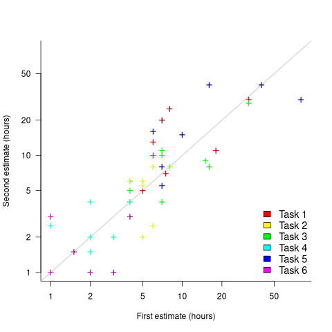
Assuming the estimation uncertainty in this experiment’s data is roughly equal to the estimation uncertainty in other estimation datasets, of tasks taking up to 20 hours, how might it be used to calculate a value for the uncertainty in estimated values?
Two possibilities include:
- Assuming that the uncertainty in both the first and second estimates is equal, a model can be fitted using Deming regression (which treats both variables as having the same uncertainty), and the residual standard error of this model used as the value of . This value for a fitted multiplicative model is 0.6 (code+data),
- using the mean of the relative errors,
}/Est_1") ; its value is 0.55.
; its value is 0.55.
How different are the models built using linear regression and errors-in-variables regression, for small task estimates?
A basic linear regression model fitted to the SiP estimation dataset is:  .
.
Updating this model, using SIMEX, to take into uncertainty in the value of  gives, for an uncertainty error of 0.55:
  , and for an uncertainty error of 0.60:
  . The coefficients for the two models are essentially the same (code+data).
The exponent value is the noticeable difference between the linear regression and errors-in-variables regression models. Adding the assumed amount of uncertainty (based on data from one experiment) to the estimated value leads to a model where estimate/actual are very close to having a linear relationship.
Is this errors-in-variables model any closer to reality than the linear regression model? The model shows that the estimate/actual relationship is closer to linear than was previously thought. Until more data becomes available, we won’t know how close this relationship actually is.
The people who made the estimates in the SiP data also performed the work that took the recorded actual time. Assigning a task to a different person could produce both a different estimate and a different actual, but these possible values are unknown. On a larger scale, different companies bidding on the same contract specify different amounts and have different implementations times; data showing these differences.
Recent Comments