Archive
Percentage of methods containing no reported faults
It is often said, with some evidence, that 80% of reported faults, for a program, occur in 20% of its code. I think this pattern is a consequence of 20% of the code being executed 80% of the time, while many researchers believe that 20% of the source code has characteristics that result in it containing 80% of the coding mistakes.
The 20% figure is commonly measured as a percentage of methods/functions, rather than a percentage of lines of code.
This post investigates the expected fraction of a program’s methods that remain fault report free, based on two probability models.
Both models assume that coding mistakes are uniformly scattered throughout the code (i.e., every statement has the same probability of containing a mistake) and that the corresponding coding mistake is contained within a single method (the evidence suggests that this is true for 50% of faults).
A simple model is to assume that when a new fault is reported, the probability that the corresponding coding mistake appears in a particular method is proportional to the method’s length,  in lines of code, of the method. The evidence shows that the distribution of methods containing a given number of lines, , is well-fitted by a power law (for Java:
  ).
).
If  reported faults have been fixed in a program containing
  methods/functions, what is the expected number of methods that have not been modified by the fixing process?
The answer (with help from: mostly Kimi, with occasional help from Deepseek (who don’t have a share chat options), ChatGPT 5, Grok, and some approximations; chat logs) is:
}Li_b(e^{-{F/M}{{zeta(b)}/{zeta(b-1)}}})")
where:  is the Riemann zeta function,
  is the polylogarithm function and
  for Java.
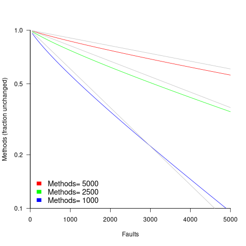
The plot below shows the predicted fraction of unmodified methods against number of faults, for programs of various sizes; the grey lines show the rough approximation:  (code+data):
The observed behavior of most reported faults involving a subset of a program’s methods can be modelled using some form of preferential attachment.
One preferential attachment model specifies that the likelihood of a coding mistake appearing in a method is proportional to ") , where
, where  is the number of previously detected coding mistakes in the method.
The estimated number of unmodified methods is now:
}Li_b(({M zeta(b-1)}/{M zeta(b-1)+a*(F+1) zeta(b)})^{1/a})")
where:  is the average value of
  over all faults (if
  , then
  for a power law with exponent 2.35).
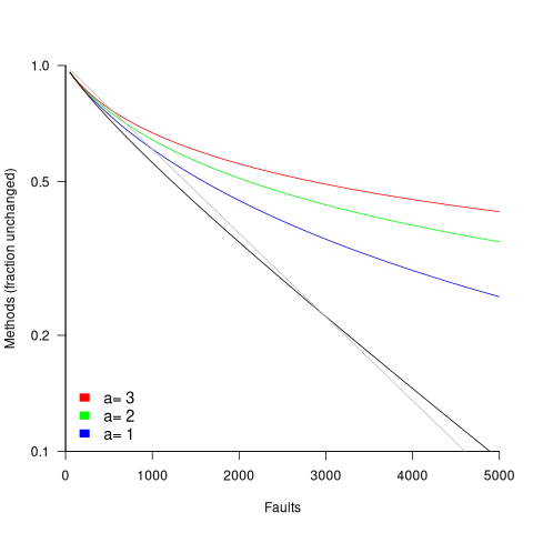
The plot below shows the predicted fraction of unmodified methods against number of faults for a program containing 1,000 methods, for various values of , with the black line showing the fraction of unmodified methods predicted by the simple model above (code+data):
In practice, random selection of the method containing a coding mistake will introduce some fuzziness in the predicted fraction of unmodified methods.
As the number of reported faults grows, the attraction of methods involved in previous reported faults slows the rate at which methods experience their first detected coding mistake.
How realistic are these models?
By focusing on the number of unmodified methods, many complications are avoided.
Both models assume that an unchanging number of methods in a program and that the length of each method is fixed. This assumption holds between each release of a program.
For actively maintained programs, the number of methods in a program changes over time, and the length of some existing methods also changes (if a program were not actively maintained, reported faults would not get fixed).
These models are unlikely to be applicable to programs with short release cycles, where there are few reported faults between releases.
How well do the models’ predictions agree with the data?
At the moment, I am not aware of a dataset containing the appropriate data. Number of faults vs unmodified methods has been added to my list of interesting patterns to notice.
Summary of the derivation of the solutions for the two models.
Simple model
The expected number of unmodified methods, ") , is:
, is:
=sum{L=1}{T}{m_L{P(U_LF)}}") , where
, where  is the length of the longest method,
  is the number of methods of length , and
 ") is the probability that a method of length will be unmodified after fault reports.
is the probability that a method of length will be unmodified after fault reports.
The evidence shows that the distribution of methods containing a given number of lines, , is well-fitted by a power law (for Java: ).
Given a program containing methods, the number of methods of length is:
 , where for Java.
If is large and  , then the sum can be approximated by the Riemann zeta function, , giving:
}}")
The probability that a method containing lines will not be modified by a fault report (assuming that fixing the mistake only involves one method) is:  , where
  is the total lines of code in the program, and the probability of this method not being modified after fault reports is approximately:
^F approx e^{{-F*L}/{P_t}}")
The expected number of empty boxes is:
}}*e^{{-F*L}/{P_t}}}=M/{zeta(b)}Li_b(e^{-F/{P_t}})")
The number of lines of code in a program containing methods is:
}}}=M/{zeta(b)}sum{L=1}{T}{L^{1-b}}=M{{zeta(b-1)}/{zeta(b)}}")
Finally giving:
}Li_b(e^{-{F/M}{{zeta(b)}/{zeta(b-1)}}})")
where is the polylogarithm function.
This equation is roughly, for the purposes of understanding the effect of each variable:

Preferential attachment model
When a mistake is corrected in a method, the attraction weight of that method increases (alternatively, the attraction weight of the other methods decreases). The probability that a method is not modified after fault reports is now:
}=prod{k=0}{F}{{P_t+a*k-L}/{P_t+a*k}}={Gamma({P_t}/a)Gamma({P_t-L}/a+F+1)}/{Gamma({P_t-L}/a)Gamma(P_t/a+F+1)}")
where:  the average value of over all faults, and
  is the gamma function.
applying the Stirling/Gamma–ratio rule, i.e., }/{Gamma(z+b)} approx z^{a-b}") we get:
we get:
})^{F/a} = ((P_t/{P_t+a*(F+1)})^{1/a})^F")
where the expression ^{1/a})^F") is the preferential attachment version of the expression
is the preferential attachment version of the expression ^F") appearing in the simple model derivation. Using this preferential attachment expression in the analysis of the simple model, we get:
appearing in the simple model derivation. Using this preferential attachment expression in the analysis of the simple model, we get:
I don’t have a rough approximation for this expression.
Preferential attachment applied to frequency of accessing a variable
If, when writing code for a function, up to the current point in the code distinct local variables have been accessed for reading  times (
 ), will the next read access be from a previously unread local variable and if not what is the likelihood of choosing each of the distinct variables (global variables are ignored in this analysis)?
Short answer:
- With probability
 select a new variable to access,
 - otherwise select a variable that has previously been accessed in the function, with the probability of selecting a particular variable being proportional to
 (where is the number of times the variable has previously been read from.
The longer answer is below as another draft section from my book Empirical software engineering with R. As always comments and pointers to more data welcome. R code and data here.
The discussion on preferential attachment is embedded in a discussion of model building.
What kind of model to build?
The obvious answer to the question of what kind of model to build is, the cheapest one that produces the desired output.
Many of the model building techniques discussed in this book find patterns in the data and effectively return one or more equations that produce output similar to the data given some set of inputs; the equations are the model.
The advantage of this approach is that in many cases the implementation of the model building has been automated (I don’t say much about those that have not yet been automated), the user contribution is in choosing which kind of model to build. In some cases the R function requires that the user provide a general direction of attack (e.g., the form of function to use in fitting a nonlinear regression).
An alternative kind of model is one whose output is obtained by running an iterative algorithm, e.g., a time series created by calculating the next value in a sequence from one or more previous values.
In most cases a great deal of domain knowledge is required of the user building the model, while in a few cases an automated procedure for creating the iterative algorithm and its parameters is available, e.g., time series analysis.
There is never any guarantee that any created model will be sufficiently accurate to be useful for the problem at hand; this is a risk that occurs in all model building exercises.
The following discussion builds two models, one using an established automated model building technique (regression) and the other using an iterative algorithm built using domain knowledge coupled with experimentation.
The problem
Consider local variable usage within a function. If a function contains a total of  read accesses to locally defined variables, how many variables will be read from only once, how many twice and so on (this is a static count extracted from the source code, not a dynamic count obtained by executing the function)?
The data for the following analysis is from Jones <book Jones_05a> (see figure 1821.5) and contains three columns, total count: the total number of read accesses to all variables defined within a function definition, object access: the number of read accesses from a distinct local variable, and occurrences: the number of distinct variables that have at least one read access within the function (i.e., unused variables are not counted); the occurrences counts have been summed over all functions.
In the following extract, within functions containing 24 totals accesses there were 783 occurrences of variables accessed once, 697 occurrences of variables accessed twice and so on.
total access,object access,occurrences 24,1,783 24,2,697 24,3,474 |
The data excludes everything about source code apart from read access information.
Fitting an equation to the data
Plotting the data shows an exponential-like decrease in occurrences as the number of accesses to a variable increases (i.e., most variables are accessed a small number of time); also there is an overall increase in the counts as the total numbers of accesses increases (see below).
The fit obtained by the nls function for a simple exponential equation is the following (all p-values less than  ; see rexample[local-use]):
where  is the number of read accesses to a given variable and is the total accesses to all local variables within the function. Because the data has been normalised the value returned is a percentage.
As an example, a function containing a total of 30 read accesses of local variables the expected percentage of variables accessed twice is:  .
.
Modeling with an incremental algorithm
If, when writing code for a function, up to the current point in the code distinct local variables have been accessed for reading times (), will the next read access be from a previously unread local variable and if not what is the likelihood of choosing each of the distinct variables (global variables are ignored in this analysis)?
Each access in the code of a local variable could be thought of as a link to the information contained in that variable. One algorithm that has been found to do a reasonable job of modeling the number of links between web pages is Preferential attachment. Might this algorithm also be applicable to modeling read accesses to local variables?
The Preferential attachment algorithm is:
- With probability
 select a new web page (in this case a new variable to access),
 - with probability
 select an existing web page (a variable that has previously been accessed in the function), select a variable with a probability proportional to the number of times it has previously been accessed (i.e., a variable that has four previous read accesses is twice as likely to be chosen as one that has had two previous accesses).
The following plot shows the results of running this algorithm 1,000 times each with 100 total accesses per function definition, for two values of (left plot 0.05, right plot 0.0004, red points) and smoothed data (blue points; smoothing involved summing the access counts for all measured functions having total accesses between 96 and 104), green line is a fitted exponential. Values have been normalised so that variables with one access have a count of 100, also access counts greater than 20 have a very low occurrences and are not plotted.
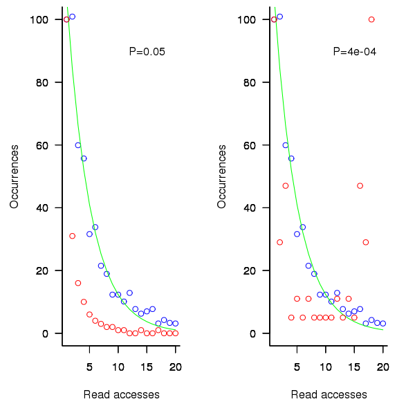
Figure 1. Variables having a given number of read accesses, given 100 total accesses, calculated from running the preferential attachment algorithm with probability of accessing a new variable at 0.05 (left, in red) and 0.0004 (right, in red), the smoothed data (blue) and a fitted exponential (green).
The results show that decreasing the probability of accessing a new variable, , does not shift the distribution of occurrences in the desired way. Note: the well known analytic solution to the outcome of running the preferential attachment algorithm, i.e., a power law, applies in the situation where the number of accesses per function definition goes to infinity.
The Preferential attachment algorithm uses a fixed probability for deciding whether to access a new variable; other measurements <book Jones_05a> imply that in practice this probability decreases as the number of distinct local variables increases. An obvious modification is to use a probability having a form something like
the number of distinct variables accessed so far). A little experimentation finds that produces results that more closely mimic the data.
While improves the fit for infrequently accessed variables, the weighting system used to select a previously accessed variable still needs attention; perhaps it also has a dependency on . Some experimentation finds that changing the probability of selection from to  (where is the number of read accesses to variable
  so far) produces behavior that matches the data to the same degree as the exponential model.
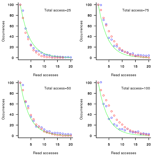
Figure 2. Variables having a given number of read accesses, given 25, 50, 75 and 100 total accesses, calculated from running the weighted preferential attachment algorithm (red), the smoothed data (blue) and a fitted exponential (green).
The weighted preferential attachment algorithm is as follows:
- With probability select a new variable to access,
- with probability
 select a variable that has previously been accessed in the function, select an existing variable with probability proportional to (where is the number of times the variable has previously been read from; e.g., if the total accesses up to this point in the code is 12, a variable that has had four previous read accesses is
  times as likely to be chosen as one that has had two previous accesses).
So what?
Both of the models are wrong in that they do not account for the small number of very frequently accessed variables that regularly occur in the data. However, as the adage goes: All models are wrong but some are useful; usefulness being evaluated by the extent to which a model solves the problem at hand. Both models have their own advantages and disadvantages, including:
- the fitted equation is quick and simple to calculate, while the output from the algorithmic model has to be averaged over many runs (1,000 are used in the example code) and is much slower,
- the algorithm automatically generates a possible sequence of accesses, while the equation does not provide an obvious way for generating a sequence of accesses,
- multiple executions of the algorithm can be used to obtain an estimate of standard deviation, while the equation does not provide a method for estimating this quantity (it may be possible to build another regression model that provides this information),
If insight into variable usage is the aim, each model provides its own particular kind of insight:
- the equation provides an end result way of thinking about how the number of variables having a given number of accesses changes, but does not provide any insight into the decision process at the level of individual accesses,
- the algorithm provides a way of thinking about how choices are made for each access, but does not provide any insight into the behavior of the final counts.
Other application domains and languages
The data used to build these models was extracted from the C source code of what might be termed desktop applications. Will the same variable access behavior characteristics occur in source written for other application domain or in other languages?
Variables might be broadly grouped into those used to hold application values (e.g., length of something) and those used to hold housekeeping values (e.g., loop counters).
Application variables are likely to be language invariant but have some dependence on algorithm (e.g., stored in an array or linked list) or cultural coding habits (e.g., within the embedded community accessing local variables is often considered to be much less efficient than accessing global variables and there are measurably different usage patterns <book Engblom_99a><book Jones 05a> figure 288.1).
The need for housekeeping values will depend on the construct supported by a language. For instance, in C loops often involve three accesses to the loop control variable to initialise, increment and test it for (i=0; i < 10; i++); in languages that support usage of the form for (i in v_list) only one access is required; in languages with vector operations many loops are implicit.
It is possible that application and language issues will change the absolute number of accesses but not effect their distribution. More measurements are needed.
Recent Comments