Archive
Programming Punched card machines
Punched card machines, or Tabulating machines, or Unit Record equipment, or according to a 1931 article Super Computing machines, were electromechanical devices that summarised information contained on punched cards (aka tabulating cards). These machines date from 1884, with the publication of Herman Hollerith’s patent application 18840923. In 1948 the electronic valve based IBM 603 calculating punch machine was launched.
The image below (from Wikipedia) shows an IBM 80 column card. When introduced in 1928, the card contained 10 rows, with rows 11 and 12 (known as zone punching positions) added later to support non-digit characters. The paper: “Do Not Fold, Spindle or Mutilate”: A Cultural History of the Punch Card takes a wry look at the social impact of these cards.

Manufacturers sold a range of single purpose Punch machines. Single purposes included: sorting cards, duplicating cards with specified changes to column contents, printing card contents, and simple accounting (adding/subtracting values).
Yes, Punched card machines can be programmed. The vast majority of machines were used by businesses for accounting and stock control, but since the early 1930s a few were used by researchers for scientific computations.
A Punch machine program consisted of cables that directed the flow of electrical signals from one to eighty output sockets (one for each of the 80 columns on a punched card), through various control/manipulation subsystems, to produce an output, e.g., printing a cheque, an itemised invoice, or creating an updated card. The input/output sockets (the terminology of the day was entry/exit sockets) for each subsystem were arranged on the machine’s Control panel (more commonly known as a plugboard).
Each plugboard contains a row of reader output sockets, one for each of the 80 card columns, a row of input sockets that connected to a printing mechanism, and sockets providing input/output for other operations. For example, a connection from, say, the 50’th column of the reader output socket to the 70’th column of the print input socket would print the contents of the 50’th column of the card in the 70’th column of the paper/card output.
The image below (from Wikipedia) shows connections for a program on an IBM 402:

Like many early computers, Punch machine architecture is bit-serial. That is, values are represented as a constant-duration sequence of bits (with the 12 rows of a column forming a card cycle), rather than a parallel sequence of bits (e.g., a byte) all appearing at the same time. The duration of the sequence is driven by the card reader, which moves the card (bottom to top) across a row of metal brushes (one for each column), completing an electric circuit (generating a pulse) when the brush makes contact through a hole in the card.
Once a card cycle completes, the bit sequences are gone (some machines could store a few column values). Some Punch machines read the same card multiple times (three is the maximum I have seen). Multiple readings make it possible to use input from the first/second reading to select the operations to be performed on the input during subsequent readings.
An example of the need for multiple reads. Holes in the zone punching positions may specify an alphabetic character or a special data specific meaning, e.g., accounting records could indicate that a column value is a credit rather than a debit by punching a hole in the 11’th row of the appropriate column. To maintain backwards compatibility, the zone punching positions appear near the top of the punch card, and are read last, leaving the digits pulses unchanged. If a zone punching position has a special meaning, the first read is used to detect whether, say, the 11’th row contains a hole, and the digit value is obtained on the second read (see X Elimination on page 126).
Punch machine programs did not support loops. Loops are implemented by including a human in the chain of execution. The body of the loop performs a calculation on the input cards, writing the results to new cards. These new cards are moved to the input hopper, and the program run again, iterating until the desired accuracy is obtained (or not).
Early research on economies of scale for computer systems
Before microprocessor cost/performance wiped out (in the early 1990s) other cpu platforms (e.g., mainframes and minis), people argued that computer hardware benefited from economies of scale.
The claimed benefit was more bang for the buck, i.e., more compute for less money.
Checking this claim requires treating pre-microprocessor computer systems and the later microprocessor-based systems as two separate cases, because many of the factors driving costs and performance are very different.
Today’s large microprocessor-based computer systems achieve economies of scale through discounts from bulk purchases and spreading fixed costs across multiple systems. The data is available, and the economic analysis is straight forward.
A lack of reliable data on the costs of designing/building pre-microprocessor computer systems rules out an economic analysis of cost/performance from first principles. The data that was/is available is the cost of computer systems and some indicators of performance (such as instruction timings or benchmarks).
Now, the observed fact that the cost of compute was decreasing over time is unrelated to the claim that the cost of compute decreases as the size of the computer increases.
Assuming a power law relationship between computer cost,  , and size,
  , at a point in time, we have:
  , where
  is some constant. Economies of scale occur when:
In his detailed cost/performance analysis of computers between 1944-1967, Kenneth Knight treated computers launched in the same year as effectively occurring at the same time. He also built a single model, with year included as an explanatory variable, which means the fitted rate of decrease is the same over all years (rather than varying between years).
The plot below uses Knight’s 1953-1961 data, and shows operations per second against seconds per dollar (a confusing combination, but what Knight used), with fitted regression lines for three years using Knight’s model (code and data)
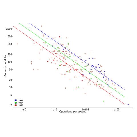
The fitted exponent for this form of x/y axis maps to a value which has , i.e., there are economies of scale.
It so happens that the value of the Knight’s fitted exponent is close to that proposed in a 1953 paper (“High speed arithmetic: The digital computer as a research tool”, no online copy):
It used to cost one cent to do a multiplication on a desk calculator; now it is more like four cents; but with these big machines we can do a million in an hour for $400, and that means twenty-five multiplications for a cent! I believe that there is a fundamental rule, which I modestly call Grosch's law, giving added economy only as the square root of the increase in speed-that is, to do a calculation ten times as cheaply you must do it one hundred times as fast. |
which did indeed become widely known as Grosch’s law.
Having been given a lucky kick-start by Knight (fitted individually, years are not close to Grosch’s law), checking for agreement with Grosch’s law became a focus for later studies. While various papers highlighted problems with the later data analysis (e.g., the regression techniques and sample noise producing mathematical artifacts), Grosch’s law ceased being a thing because mainframes/minicomputers ceased being a thing.
Did mainframe/mincomputers have economies of scale in the years after Knight’s data? It’s difficult to tell, the publicly available data is too sparse to support reliable analysis.
Data+code for book: The New C Standard
All the data+code from my book The New C Standard: An Economic and Cultural Commentary is now available on GitHub. For many years I have been meaning to create an easy way to map from a graph/table in the book to the file containing the data, which has blocked me adding the data to GitHub. I have unblocked by releasing this minimal viable product, i.e., it is essentially a copy of the usage subdirectory in the book’s directory.
While the five stage process to get from graph/table to data is tedious, at least there is a process that provides the data. The caption of the graphs in my Evidence-based Software Engineering book contain a link to the corresponding file on GitHub. This was not possible for the C book because GitHub was still 3-years in the future when the book was published (in 2005).
Work on the book started in late 1999 and measurements of C usage was an integral component. Publicly available source code was still a novelty and large Open source projects were rare (SourceForge was launched at the end of 1999). The large projects with C source available to measure were: Linux, Netscape, Gcc, PostgresSQL, OpenAFS, and OpenMotif. Several popular projects originally written in C had migrated to using C++, and were therefore not applicable.
As the book was completed in 2005, evidence-based software engineering restarted, 20-years after the fall of Rome. Or rather, I have nominated 2005 as the year this happened. Feel free to quibble plus/minus a few years.
Search engines were an essential tool for obtaining research papers, reports, and occasionally downloading data. In 2000 the search engine of choice was AltaVista, but a few years later Google had become the best.
While writing the book, I was a regular visitor to bricks and mortar buildings called libraries. Back then, university libraries contained tens of thousands of physical books, and researchers would photocopy papers of interest. Little did I know that this research practice would soon be dead.
In 2005, I had this to say about software evolution:
Measuring the characteristics of software that change over many releases (software evolution) is a relatively new research topic. Software evolution is discussed in a few sentences, and any future major revision ought to cover this important topic in substantially more detail. |
How might C source code characteristics have changed in the last 20 years?
- The use of K&R style function definitions is probably very rare; it was well on the way out in 1999,
- big software systems have gotten bigger, i.e., more lines of code and more
#includes, - A lot more code using 32-bit integers and 64-bit pointers,
- More storage allocated (memory capacity has increased) because it’s faster to do everything in memory, and there is more data.
After 55.5 years the Fortran Specialist Group has a new home
In the 1960s and 1970s, new developments in Cobol and Fortran language standards and implementations regularly appeared on the front page of the weekly computer papers (Algol 60 news sometimes appeared). Various language user groups were created, which produced newsletters and held meetups (this term did not become common until a decade or two ago).
In January 1970 the British Computer Society‘s Fortran Specialist Group (FSG) held its first meeting and 55.5 years later (this month) this group has moved to a new parent organization the Society of Research Software Engineering. The FSG is distinct from BSI‘s Fortran Standards panel and the ISO Fortran working group, although they share a few members.
I believe that the FSG is the oldest continuously running language user group. Second place probably goes to the ACCU (Association on C and C++ Users) which was started in the late 1980s. Like me, both of these groups are based in the UK (the ACCU has offshoots in other countries). I welcome corrections from readers familiar with the language groups in other countries (there were many Pascal user groups created in the 1980s, but I don’t know of any that are still active). COBOL is a business language, and I have never seen a non-vendor meetup group that got involved with language issues.
The plot below shows estimated FSG membership numbers for various years, averaging 180 (thanks to David Muxworthy for the data; code+data):

My experience of national user groups is that membership tends to hover around a thousand. Perhaps the more serious, professional approach of the BCS deters the more casual members that haunt other user groups (whose membership fees help keep things afloat).
What are the characteristics of this Fortran group that have given it such a long and continuous life?
- It was started early. Fortran was one of the first, of two (perhaps three), widely used programming languages,
- Fortran continued to evolve in response to customer demand, which made it very difficult for new languages to acquire a share of Fortran’s scientific/engineering market. Compiler vendors have kept up, or at least those selling to high-end power customers have (the Open source Fortran compilers have lagged well behind).
Most developers don’t get involved with calculations using floating-point values, and so are unfamiliar with the multitude of issues that can have a significant impact on program output, e.g., noticeably inaccurate results. The Fortran Standard’s committee has spent many years making it possible to write accurate, portable floating-point code.
A major aim of the 1999 revision of the C Standard was to make its support for floating-point programming comparable to Fortran, to entice Fortran developers to switch to C,
- people being willing to dedicate their time, over a long period, to support the activities of this group.
The minutes of all the meetings are available. The group met four times a year until 1993, and then once or twice a year. Extracting (imperfectly) the attendance from the minutes finds around 525540 unique names, with 322350 attending once and one person attending 8155 meetings. The plot below shows the number of people who attended a given number of meetings (code+data):

The survival of any group depends on those members who turn up regularly and help out. The plot below shows a sorted list of FSG member tenure, in years, excluding single attendance members (code+data):

Will the FSG live on for another 55 years at the Society of Research Software Engineering?
Fortran continues to be used in a wide range of scientific/engineering applications. There is a lot of Fortran source out there, but it’s not a fashionable language and so rarely a topic of developer conversation. A group only lives because some members invest their time to make things happen. We will have to wait and see if this transplanted groups attracts a few people willing to invest in it.
Update the next day. Added attendance from pdf minutes, and removed any middle initials to improve person matching.
The inconvenient history of Liberal Fascism
Based purely on its title, Liberal Fascism: The secret history of the Left from Mussolini to the Politics of Meaning by Jonah Goldberg, published in 2007, is not a book that I would usually consider buying.
The book traces the promotion and application of fascistic ideas by activists and politicians, from their creation by Mussolini in the 1920s to the start of this century. After these ideas first gained political prominence in the 1920s/30s as Fascism, they and the term Fascism became political opposites, i.e., one was adopted by the left and the other labelled as right-wing by the left.
The book starts by showing the extreme divergence of opinions on the definition of Fascism. The author’s solution to deciding whether policies/proposals are Fascist to compare their primary objectives and methods against those present (during the 1920s and early 1930s) in the policies originally espoused by Benito Mussolini (president of Italy from 1922 to 1943), Woodrow Wilson (the 28th US president between 1913-1921), and Adolf Hitler (Chancellor of Germany 1933-1945).
Whatever their personal opinions and later differences, in the early years of Fascism Mussolini, Wilson and Hitler made glowing public statements about each other’s views, policies and achievements. I had previously read about this love-in, and the book discusses the background along with some citations to the original sources.
Like many, I had bought into the Mussolini was a buffoon narrative. In fact, he was extremely well-read, translated French and German socialist and philosophical literature, and was considered to be the smartest of the three (but an inept wartime leader). He was acknowledged as the father of Fascism. The Italian fascists did not claim that Nazism was an offshoot of Italian fascism, and went to great lengths to distance themselves from Nazi anti-Semitism.
At the start of 1920 Hitler joined the National Socialist party, membership number 555. There is a great description of Hitler: “… this antisocial, autodidactic misanthrope and the consummate party man. He has all the gifts a cultist revolutionary party needed: oratory, propaganda, an eye for intrigue, and an unerring instinct for populist demagoguery.”
Woodrow Wilson believed that the country would be better off with the state (i.e., the government) dictating how things should be, and was willing for the government to silence dissent. The author describes the 1917 Espionage Act and the Sedition Act as worse than McCarthyism. As a casual reader, I’m not going to check the cited sources to decide whether the author is correct and that the Wikipedia articles are whitewashing history (he does not claim this), or that the author is overselling his case.
Readers might have wondered why a political party whose name contained the word ‘socialist’ came to be labelled as right-wing. The National Socialist party that Hitler joined was a left-wing party, i.e., it had the usual set of left-wing policies and appealed to the left’s social base.
The big difference, as perceived by those involved, between National Socialism and Communism, as I understand it, is that communists seek international socialism and define all nationalist movements, socialist or not, as right-wing. Stalin ordered that the term ‘socialism’ should not be used when describing any non-communist party.
Woodrow Wilson died in 1924, and Franklin D. Roosevelt (FDR) became the 32nd US president, between 1933 and 1945. The great depression happens and there is a second world war, and the government becomes even more involved in the lives of its citizens, i.e., Mussolini Fascist policies are enacted, known as the New Deal.
History repeats itself in the 1960s, i.e., Mussolini Fascist policies implemented, but called something else. Then we arrive in the 1990s and, yes, yet again Mussolini Fascist policies being promoted (and sometimes implemented) under another name.
I found the book readable and enjoyed the historical sketches. It was an interesting delve into the extent to which history is rewritten to remove inconvenient truths associated with ideas promoted by political movements.
Christmas books for 2024
My rate of book reading has picked up significantly this year. The following are the really interesting books I read, as is usually the case, most were not published in this year.
I have enjoyed Grayson Perry’s TV programs on the art world, so I bought his book “Playing to the Gallery: Helping Contemporary Art in its Struggle to Be Understood“. It’s a fun, mischievous look at the art world by somebody working as a traditional artist, in the sense of creating work that they believe means/says something, rather than works that are only considered art because they are displayed in an art gallery.
“The Computer from Pascal to von Neumann” by H. H. Goldstine. This history of computing from the mid-1600s (the time of Blaise Pascal) to the mid-1900s (von Neumann died in 1957) told by a mathematician who was first involved in calculating artillery firing tables during World War II, and then worked with early computers and von Neumann. This book is full of insights that only a technical person could provide and is a joy to read.
I saw a poster advertising a guided tour of the trees in my local park, organized by Trees for Cities. It was a very interesting lunchtime; I had not appreciated how many different trees were growing there, including three different kinds of Oak tree. Trees for Cities run events all over the UK, and abroad. Of course, I had to buy some books to improve my tree recognition skills. I found “Collins tree guide” by O. Johnson and D. More to be the most useful and full of information. Various organizations have created maps of trees in cities around the world. The London Tree Map shows the location and species information for over 880,000 of trees growing on streets (not parks), New York also has a map. For a general analysis of patterns of tree growth, see “How to Read a Tree” by T. Gooley.
“Medieval Horizons: Why the Middle Ages Matter” by I. Mortimer. This book takes the reader through the social, cultural and economic changes that happened in England during the Middle Ages, which the author specifies as the period 1000 to 1600. I knew that many people were surfs, but did not know that slaves accounted for around 10% of the population, dropping to zero percent during this period. Changes, at least for the well-off, included moving from living in longhouses to living in what we would call a house, art works moved from two-dimensional representations to life-like images (e.g., renaissance quality), printing enables an explosion of books, non-poor people travelled more, ate better, and individualism started to take-off.
Statistical Consequences of Fat Tails: Real World Preasymptotics, Epistemology, and Applications by N. N. Taleb is a mathematically dense book (while the pdf is in color, I was disappointed that the printed version is black/white; this is the one I read while travelling). This book tells you a lot more than you need to know about the consequences of fat tail distributions. Why might you be interested in the problems of fat tails? Taleb starts by showing how little noise it takes for the comforting assumptions implied by the Normal/Gaussian distribution to fly out the window. The primary comforting assumptions are that the mean and variance of a small sample are representative of the larger population. A world of fat tail distributions is one where the unexpected is to be expected, where a single event can wipe out an organization or industry (banks are said to have lost more in the 2008 financial crisis than they had made in the previous many decades). This book is hard going, and I kept at it to get a feel for the answers to some of the objections to the bad news conveyed. There are a couple of places where I should have been more circumspect in my Evidence-based software engineering book.
I have previously reviewed General Relativity: The Theoretical Minimum by Susskind and Cabannes.
“Embracing Defeat: Japan in the Wake of World War II” by John W. Dower describes in harrowing detail the dire circumstances of the population of Japan immediately after World War II and what they had to endure to survive.
For more detailed book reviews, see: Mr. and Mrs. Psmith’s Bookshelf with some excellent and insightful long book reviews, and the annual Astral Codex Ten book review contest usually has a few excellent reviews/books.
For those of you who think that civilization is about to collapse, or at least like talking about the possibility, a reading list. At the practical level, I think sword fighting and archery skills are more likely to be useful in the longer term.
21 Algol 60 compilers in 1962
The specification of ALGOL 60 was published in May 1960. Unlike today, where the creators of a new language release the source of a corresponding compiler, people were expected to write their own compiler. The June 1962 paper: The Replies to the AB14 Questionnaire lists implementation details on 21’ish compilers (it’s not clear whether some are dialects or languages very similar to Algol 60; 1963: list of 32 Algol compilers/versions).
Compiler writing was a hot leading edge research topic in the 1960s; at the start of this decade all the techniques we take for granted today had not yet been invented (Knuth invented LR parsing in 1965, and algorithms for optimal code generation started appearing in 1970). The 1960s was the period of the Cambrian explosion for programming languages.
Implementors not only had to deal with all the unknowns of writing a compiler, they also had to do the work using systems whose memory was measured in tens of kilobytes, computer interaction probably via punched card or punched tape, or if lucky, the luxury of teletype input/output. It’s no surprise that fourteen of the implementations considered themselves to be a “true subset” (which I take to mean that everything implemented was as per the specification). Compilers for earlier languages probably had the benefit of the language not supporting anything that was hard to implement.
Compiler implementation know-how received a major boost in 1964 with the publication of the book ALGOL 60 Implementation.
The plot below shows the number of compilers having a given reported implementation time (code+data):
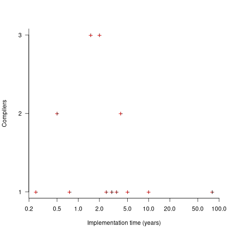
The median implementation effort is 2 man-years. Is this the result of a few good people working off the clock to create software, or management supporting the creation of a product that customers are not clamouring for?
The 0.25 man-year implementation looks like a port of an existing compiler to a different version of the same hardware. The 10 man-year implementation time was for what looks like a full implementation, plus extensions. The 80 man-year implementation time was reported by SDC (a large defence contractor) for a range of JOVIAL compilers (derived from Algol 58) targetting five different hardware platforms.
Were the implementors of Algol compilers different from the implementors of other languages? It’s not possible to say, although the language was created by a distinct group of people. The definition of Algol 60 was created by a committee composed of computing academics and like-minded people, while Fortran was dominated by the major computer company of the day, IBM (1963: list of 51 Fortran compilers; 1964: at least 43 Fortran compilers/versions), and COBOL was designed to be used by those strange business people (1963: list of 37 COBOL implementations/versions).
The Norden-Rayleigh model: some history
Since it was created in the 1960s, the Norden-Rayleigh model of large project manpower has consistently outperformed, or close runner-up, other models in benchmarks (a large project is one requiring two or more man-years of effort). The accuracy of the Norden-Rayleigh model comes with a big limitation: a crucial input value to the calculation is the time at which project manpower peaks (which tends to be halfway through a project). The model just does not work for times before the point of maximum manpower.
Who is the customer for a model that predicts total project manpower from around the halfway point? Managers of acquisition contracts looking to evaluate contractor performance.
Not only does the Norden-Rayleigh model make predictions that have a good enough match with reality, there is some (slightly hand wavy) theory behind it. This post delves into Peter Norden’s derivation of the model, and some of the subsequent modifications. Norden work is the result of studies carried out at IBM Development Laboratories between 1956 and 1964, looking for improved methods of estimating and managing hardware development projects; his PhD thesis was published in 1964.
The 1950s/60s was a period of rapid growth, with many major military and civilian systems being built. Lots of models and techniques were created to help plan and organise these projects, two that have survived the test of time are the critical path method and PERT. As project experience and data accumulated, techniques evolved.
Norden’s 1958 paper “Curve Fitting for a Model of Applied Research and Development Scheduling” describes how a project consists of overlapping phases (e.g., feasibility study, deign, implementation, etc), each with their own manpower rates. The equation Norden fitted to cumulative manpower was:  , where
  is project elapsed time,
  is total project manpower, and ,
  , and
, and  are fitted constants. This is the logistic equation with added tunable parameters.
By the early 1960s, Norden had brought together various ideas to create the model he is known for today. For an overview, see his paper (starting on page 217): Project Life Cycle Modelling: Background and Application of the Life Cycle Curves.
The 1961 paper: “The decisions of engineering design” by David Marples was influential in getting people to think about project implementation as a tree-like collection of problems to be solved, with decisions made at the nodes.
The 1958 paper: The exponential distribution and its role in life testing by Benjamin Epstein provides the mathematical ideas used by Norden. The 1950s was the decade when the exponential distribution became established as the default distribution for hardware failure rates (the 1952 paper: An Analysis of Some Failure Data by D.J. Davis supplied the data).
Norden draws a parallel between a ‘shock’ occurring during the operation of a device that causes a failure to occur and a discovery of a new problem to be solved during the implementation of a task. Epstein’s exponential distribution analysis, along with time dependence of failure/new-problem, leads to the Weibull distribution. Available project manpower data consistently fitted a special case of the Weibull distribution, i.e., the Rayleigh distribution (see: Project Life Cycle Modelling: Background and Application of the Life Cycle Curves (starts on page 217).
The Norden-Rayleigh equation is:  , where:
  is work completed, is total manpower over the lifespan of the project,
  ,
,  is time of maximum effort per unit time (i.e., the Norden/Rayleigh equation maximum value), and is project elapsed time.
Going back to the original general differential equation, before a particular solution is obtained, we have: *(1-W(t))") , where
, where ") is the amount of work left to do (it’s sometimes referred to as the learning curve). Norden assumed that:
is the amount of work left to do (it’s sometimes referred to as the learning curve). Norden assumed that: =a*t") .
.
The 1980 paper: “An alternative to the Rayleigh curve model for software development effort” by F.N. Parr argues that the assumption of work remaining being linear in time is unrealistic, rather that because of the tree-like nature of problem discovery, the work still be to done, , is proportional to the work already done, i.e., =beta*W(t)") , leading to:
, leading to: ") , where: is some fitted constant.
, where: is some fitted constant.
While the Norden-Rayleigh equation looks very different from the Parr equation, they both do a reasonable job of fitting manpower data. The following plot fits both equation to manpower data from a paper by Basili and Beane (code+data):

A variety of alternative forms for the quantity have been proposed. An unpublished paper by H.M. Hubey discusses various possibilities.
Some researchers have fitted a selection of equations to manpower data, searching for the one that gives the best fit. The Gamma distribution is sometimes found to provide a better fit to a dataset. The argument for the Gamma distribution is not based on any theory, but purely on the basis of being the best fitting distribution, of those tested.
The 2024 update to my desktop system
I have just upgraded my desktop system. As you can see from the picture below, it is a bespoke system; the third system built using the same chassis.
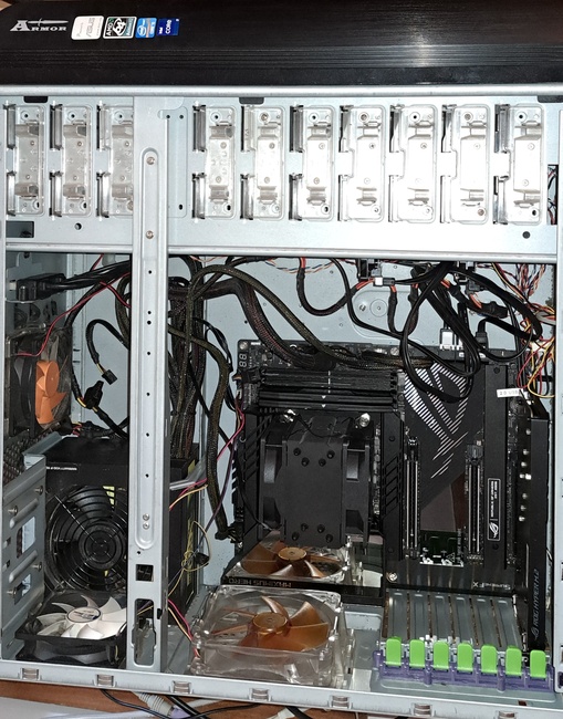
The 11 drive bays on the right are configured for six 5.25-inch and five 3.5-inch disks/CD/DVD/tape drives, there is a drive cage that fits above the power supply (top left) that holds another three 3.5-inch devices. The central black rectangle with two sets of four semicircular caps (fan above/below) is the cpu cooling tower, with two 32G memory sticks immediately to its right. The central left fan is reflected in a polished heatsink.
Why so many bays for disks?
The original need, in 2005 (well before GitHub), was for enough storage to hold the source code available, via ftp, from various hosting sites that were springing up, hence the choice of the Thermaltake Armour Series VA8000BWS Supertower. The first system I built contained six 400G Barracuda drives
The original power supply, a Thermaltake Silent Purepower 680W PSU, with its umpteen power connectors is still giving sterling service (black box with black fan at top left).
When building a system, I start by deciding on the motherboard. Boards supporting 6+ SATA connectors were once rare, but these days are more common on high-end systems. I also look for support for the latest cpu families and high memory bandwidth. I’m not a gamer, so no interest in graphics cards.
The three systems are:
- in 2005, an ASUS A8N-SLi Premium Socket 939 Motherboard, an AMD Athlon 64 X2 Dual-Core 4400 2.2Ghz cpu, and Corsair TWINX2048-3200C2 TwinX (2 x 1GB) memory. A Red Hat Linux distribution was installed,
- in 2013, an intermittent problem appeared on the A8N motherboard, so I upgraded to an ASUS P8Z77-V 1155 Socket motherboard, an Intel Core i5 Ivy Bridge 3570K – 3.4 GHz cpu, and Corsair CMZ16GX3M2A1600C10 Vengeance 16GB (2x8GB) DDR3 1600 MHz memory. Terabyte 3.25-inch disk drives were now available, and I installed two 2T drives. A openSUSE Linux distribution was installed.
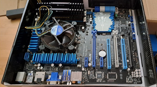
The picture below shows the P8Z77-V, with cpu+fan and memory installed, sitting in its original box. This board and the one pictured above are the same length/width, i.e., the ATX form factor. This board is a lot lighter, in color and weight, than the Z790 board because it is not covered by surprisingly thick black metal plates, intended to spread areas of heat concentration,
- in 2024, there is no immediate need for an update, but the 11-year-old P8Z77 is likely to become unreliable sooner rather than later, better to update at a time of my choosing. At £400 the ASUS ROG Maximus Z790 Hero LGA 1700 socket motherboard is a big step up from my previous choices, but I’m starting to get involved with larger datasets and running LLMs locally. The Intel Core i7-13700K was chosen because of its 16 cores (I went for a hefty cooler upHere CPU Air Cooler with two fans), along with Corsair Vengeance DDR5 RAM 64GB (2x32GB) 6400 memory. A 4T and 8T hard disk, plus a 2T SSD were added to the storage system. The Linux Mint distribution was installed.
The last 20-years has seen an evolution of the desktop computer I own: roughly a factor of 10 increase in cpu cores, memory and storage. Several revolutions occurred between the roughly 20 years from the first computer I owned (an 8-bit cpu running at 4 MHz with 64K of memory and two 360K floppy drives) and the first one of these desktop systems.
What might happen in the next 20-years?
Will it still be commercially viable for companies to sell motherboards? If enough people switch to using datacenters, rather than desktop systems, many companies will stop selling into the computer component market.
LLMs perform simple operations on huge amounts of data. The bottleneck is transferring the data from memory to the processors. A system where simple compute occurs within the memory system would be a revolution in mainstream computer architecture.
Motherboards include a socket to support a specialised AI chip, like the empty socket for Intel’s 8087 on the original PC motherboards, is a reuse of past practices.
A new NASA software dataset from the 1970s
When modeling the process of software development, to optimise the creation of new projects, the best measurement data to use are those relating to whatever developers are doing today.
Unfortunately, measurement data for software engineering processes is very hard to find; few development groups record anything about what they do, and even when they do the files are rarely kept.
Anybody involved in evidence-based software engineering has to be willing to work with whatever data is available, even when it is for software systems built decades ago.
The usefulness of any measurement data, ancient or recent, is dependent on its relevance to the questions being analysed.
During a recent search for the DACS dataset, I found measurement data for 29 software projects contained in a 1981 NASA report. While the projects happened decades ago (1975-1981) for a niche application (software for spacecraft), the measurement data is much more extensive than usual, containing background information on many of the projects; given the rarity of software project data from this period, the 47 rows of data on each project, in Table 3.1-1, looked interesting enough to extract and analyse (output from Amazon’s usually robust Textract needed some hours of manual post-processing; code+data).
While this data is not of immediate use, I will invariably get involved in a discussion, or analysis, where this dataset will be a big improvement on nothing.
Are there any points to note?
- there is a linear relationship between the totals of programmer hours and management hours, with an average of 4.4 programmer hours per management hour. This sounds low, but these projects are developing embedded software and there are likely to be many stakeholders,
- the average percentage of time spent in each phase of the Waterfall process used was: Design 31%, Code-Test 29%, System testing 11%, Acceptance testing 10%, Cleanup 20%. Lots of testing is to be expected for spacecraft software,
- the average number of project source lines was 34k. I don’t know whether this is high or low, NASA press releases invariably cite the total amount of code on the spacecraft.
It’s worth noting that this small dataset is of a size and project detail that was used by researchers in the 1970s/1980s to validate software theories that are still with us today, e.g., the COCOMO estimation model, the McCabe metrics were not validated on any data, and the Halstead metrics were checked using multiple datasets each of similar size. I suspect that many of these datasets also came from DOD or NASA projects.
Recent Comments