The Shape of Code

For some time I have been looking for a good example to illustrate the difference between predicting some software attribute and controlling that attribute. A recent study comparing two methods of predicting a person’s height looks like it might be what I am after.

The study compared the accuracy of using information derived from a person’s genes to information on their parents’ height.

If a person is not malnourished or seriously ill while growing, then their genes control how tall they will finish up as an adult. Tinker with the appropriate genes while a person is growing and their final height will be different; tinker after they have reached adulthood and height is unlikely to change,

Around 150 years ago Francis Galton developed a statistical technique that enabled a person’s final adult height to be estimated from their parent’s height. Parent height is a predictor, not a controller, of their children’s height.

A few metrics have been found empirically to correlate with faults in code and a larger number, having no empirical evidence of a correlation, have been proposed as fault ‘indicators’. Unfortunately many software developers and most managers are blind to the saying “correlation does not imply causation”.

I’m sure readers would agree that once a baby is born changes to their parents height has no effect on their final adult height. Following this line of argument we would not expect changing source code to reduce the number of faults predicted by some metric to actually reduce the number of faults (ok, fiddling with the source might result in a fault being spotted and fixed).

The interesting part of the study was the finding that the prediction based on existing knowledge about the genetics of height explained 4-6% of subjects’ sex- and age-adjusted height variance, while Galton’s method based on parent height explained 40%. Today, 60 years after the structure of DNA was discovered our knowledge of what actually controls height is nowhere near as encompassing as an attribute that is purely a predictor.

Today, do we have have a good model of what actually happens when code is written? I think not.

How much time and money is being wasted changing software to improve its fit to predictor metrics rather than control metrics (I have little idea what any of these might be)? I dread to think.

People look for patterns and expect others to follow patterns of behavior. Some preliminary data from a game of Colonel Blotto run by a group of Cornell University graduate students provides a vivid example of the existence of these behavior patterns.

In the Cornell implementation of the Colonel Blotto game, there are 10 fields and 100 soldiers. A player specifies how many soldiers are posted to each of the 10 fields. Players don’t know what the opposing players will do. In each field the battle is decided by whoever has the most soldiers with equal numbers resulting in a draw. Whoever wins the most battles wins the war.

One possible soldiers per field sequence is 10 10 10 10 10 10 10 10 10 10 and another is 1 11 11 11 11 11 11 11 11 11. The second sequence will lose in the first field, but win the other 9, and therefore win the war. A third sequence is 9 11 12 12 12 12 8 8 8 8 which beats the second sequence but only draws against the first.

The number of ways of placing indistinguishable soldiers into fields is:

The following original analysis assumes that the soldiers are distinguishable, which they are not and so the number calculated is way too large (thanks to Forbes at The Virtuosi for pointing this out): There are 10 ways of placing the first soldier, 10 ways of placing the second and so on, giving possible arrangements.

Some arrangements obviously always lose (25 25 25 25 0 0 0 0 0 0) and won’t be played; it seems reasonable to assume that no field will contain zero (I will talk about putting 0 in one field later), so having a field contain 1 is a draw at best. Lets assume that all fields contain at least 2 soldiers, which means we have 80 left to arrange giving possibilities; a very big drop in possibilities but still a huge number.

The more soldiers appearing in a field the more likely a win will occur there, but after a while the law of diminishing returns kicks in and losses occurring in understaffed fields will be greater. Lets assume that people decide never to put more than 20 soldiers in a field; how many possibilities does this rule out? If one field initially contains 21 soldiers and the others 2 each the remaining 61 soldiers create unused possibilities, putting 21 soldiers in the second field generates a bit less than new possibilities; lets round up and say there are a total of unused possibilities. Compared to the unused is small enough to be ignored.

is such a big number that Chimpanzees randomly typing away since the dawn of time are unlikely to create any discernible pattern in the landscape.

If the players in this game had given random answers what would be the mean number of points scores and its variance?

Comparing the soldier sequence given by player A against the sequence given by player B produces 11 possible scores, {0, 10}, {1, 9} … {5, 5} … {10, 0}, five of them resulting in a win for A, five in a win for B and one in a draw. With 2 points for a win, 1 point for a draw and 0 points for a loss the expected number of points for each of the two players is 1, so for players the expected mean of each player is . In a game containing 550 players (the number that had played when I extracted the score results today; 347 had played in the preliminary Cornell data set) we would expect the average score to be 550.

The variance can be calculated from:

The standard deviation about our mean is or 22.4.

Plotting a histogram of points scored, at the time of writing, we get the following:

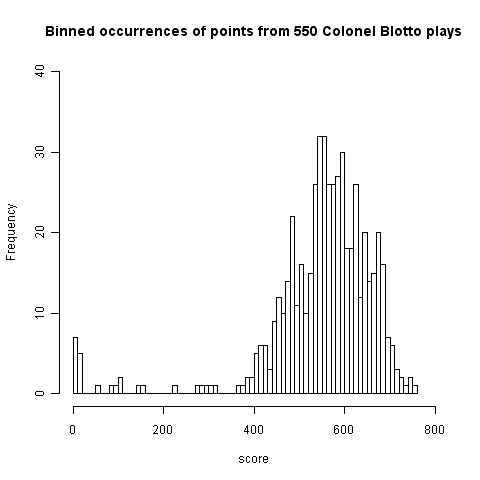
This has a peak at 550 where we would expect it and its width is two standard deviations 🙂 However those ‘side-lobes’ were not expected and they are asymmetric. I think the reason for these unexpected ‘side-lobes’ is that some players give multiple answers, attempting to improve their ranking (some strategy name are suggestive of retries with modified strategies) and consequently decreasing the total points of other players. A search space of sequences is so large that we would not expect players to be able to learn from the results of previously submitted sequences unless many of the previously submitted sequences followed some pattern that they could recognise.

What pattern of behavior might players follow? I can imagine players starting low/high and then shifting to high/low, perhaps following this sequence two or more times.

A preliminary summary of some of the data seen so far by Alex Alemi gave me enough information to figure out a sequence, in three attempts, that ranked 1st (a typo on my part prevented it being on the second attempt); my sequence of player names is averages, aver_p6, low_high_dip, followed by a bit of tuning: low_high_dipish, lohilohi_slide, followed by two experiments: the_well, heat_map, and user fooly started getting close and I tuned the sequence a bit more lohilohi_sliiide.

I used the sequences from the top 25 ranked players for my analysis and did not make any attempt to deduce other player patterns. My first attempt averaged the number of soldiers in each field, ranked 62nd as I write (aver_p6). Then I spotted that several distribution patterns existed, I picked what looked like the most promising and averaged over it (by eye) to get the then current to number 1 (currently languishing in 8th).

Had I put a bit more thought into things I could also have used the heat map near the bottom of the post (thanks to Alex Alemi for letting me post a copy here; “With Y soldiers in slot X, what percentage of the existing strategies do you beat in slot X.”):

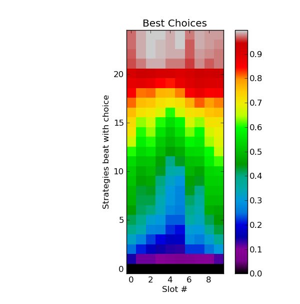
This shows one pattern (in light blue) where players are following the pattern low-high-low-high-low with the second low being very precipitous. The patterns visible in green are more complicated, but still contain a recurring low-high theme.

I know next to nothing about autocorrelation and so do not have any bright ideas about how to use of this data to improve my score. The heat_map sequence (7 8 9 12 15 16 9 11 7 6) attempts to follow the light blue pattern and is ranked 296 as I write, just under half way down the rankings and something to be expected from following an average.

Once a major pattern has been deduced ‘extra’ soldiers will be needed to outnumber the other players most of the time. One option is to be willing to always lose in one field (e.g., the one usually requiring the most soldiers) and use the freed up resources to win elsewhere. I have only made one attempt using this strategy (the_well: 5 6 7 11 19 0 14 20 13 5, ranked 72 as I write).

It is possible that common patterns of behavior are created through reinforcement. Early players create an initial configuration of results and slightly later players attempt to find it, perhaps visualizing a pattern where none actually exists. If enough people follow the same trail they will create the pattern that others can will try to follow. Results from other Colonel Blotto games exhibit a pattern of behavior that is different from the one in the Cornell dataset (I have only seen what is publicly available)

Many coding guidelines recommend against the presence of unreachable code in source; the argument being that while the code itself is harmless its presence suggests something has gone wrong somewhere else. As a member of the MISRA C++ coding guidelines committee I unsuccessfully argued against this recommendation being included on the grounds of lack of evidence that unreachable code was a significantly strong indicator of a fault and the complications caused by wanting allow certain kinds of what appeared to be unreachable code (e.g., that used by defensive programming practices).

I was recently reading the PhD thesis of Yichen Xie and found some very interesting analysis of correlation between various kinds of dead code (redundant code was one of the kinds) and faults.

Yichen Xie took a course grained approach to finding a correlation between redundant code and faults. He simply counted the numbers of files that did/did not contain redundant code and the number of corresponding files known to contain what he called a hard bug. The counts were as follows (statistical analysis using the contingency table method gives a probability of well below 0.01 for these values being generated by the null hypothesis):

               Hard Bugs
Dead Code     Yes     No   Totals
  Yes         133     135    268
   No         418    1369   1787
Totals        551    1504   2055

These counts show that if one of the 2,055 files was picked at random the expectation of it containing a Hard Bug is 27%, for one of the files containing unreachable code the expectation is 50% and for files not containing unreachable code it is 23%. So picking a file containing unreachable code almost doubles the expectation of a Hard Bug being found in that file.

These measurements do not attempt to make a connection between the unreachable code contained in a file and any fault contained within that file. How would the counts change if they were based on their being some form of logical connection between the redundant code and the fault? The counts suggest at least a 50% false positive rate, but then faults that generate unreachable code may be the result of high level semantic issues that are less likely to be detected by a casual reading of the source or by static analysis tools.

The hoped for consequence of a coding guideline requiring the removal of unreachable code is that developers analyze the code to understand why the code is unreachable and that in many cases this will result in a fault being uncovered and fixed; the worst case scenario is that they simply delete the unreachable code.

This research has caused me to upgrade the significance I give to unreachable code but I remain unconvinced that the false positive rate is sufficiently low for it to be a worthwhile coding guideline.

An interesting paper on untangling skill and luck in sports and business made the interesting observation that if, for some activity, it is easy to lose on purpose then skill dominates over luck, while if it is difficult to lose on purpose luck dominates over skill.

This got me thinking about skill in software development and how it might be used to ‘loose on purpose’ (I will leave the question of luck in software development to another post).

What does winning and loosing mean in software development? Winning might mean producing a program quickly, cheaply, that is the most efficient or is the most maintainable. I’m not sure that there is much skill involved in being the slowest or most expensive developer to write code, or to create a very inefficient program.

Everybody has ideas about how to write maintainable code (there is generally little or no experimental evidence to back up these ideas) and from time to time joke articles about writing unmaintainable code are written.

There are practical reasons for wanting to create non-maintainable or difficult to comprehend code, for instance to make it difficult for a third party (who might be a customer or black hat) to figure out how a program operates. So called obfuscating transformations are an active area of research and tools are available to transform source and binary; the effectiveness of some techniques for making source difficult to maintain is debatable and obfuscating source may have little impact on the generated binary.

These tools primarily operate by removing information, e.g., rewriting identifiers to meaningless sequences of characters, mapping structured loops to sequences of goto and folding constant expressions. Removing information does not require any skill relating to software maintainability.

I would claim that being able to add negative information to a program is evidence of skill for software maintenance.

Some example of the kinds of negative information I would add include:

• Invented ‘magic’ numbers, i.e., numeric literals that look as if they are derived from an application domain requirement. For instance, a reader of the expression x*12 is likely to assume that 12 is a constant specific to some aspect of the application; this is an instance where novice developers are trained to invent a symbolic name (e.g., max_eggs_in_box) to denote the given value. So if the original code contained the expression x*6 I would modify it to x*12 and then figure out how to later divide the result by two. Code modified to contain many 12s, or other such ‘invented’ constants, is likely to cause readers to waste lots of time head scratching.
• Replace identifiers with names that have no semantic connection with the information they contain. Well chosen identifier names can significantly reduce the effort needed to comprehend source and I’m sure that suitable chosen names would help sow lots of confusion. An experiment I ran a few years ago found that developers use identifier names to make decisions about binary operator precedence; lots of scope for creating confusion here!
• I don’t have enough experience to know whether restructuring class hierarchies will have a worthwhile impact on maintainability, developers have learned to handle poorly designed class hierarchies and I am not sure I can make things much worse than they have already encountered.

Adding redundant code is a commonly used technique. To be effective this code would have to modify variables used in the original program, which means that it would have to occur in a condition that is never executed; a constant conditional expression would fool nobody and the condition would have to rely on a variable being tested against a value that could never occur. This requires application knowledge not code maintenance skills.

Compression and encryption (of strings in source and as much code as possible in executables) are other existing techniques that do not involve maintenance related skills.

While reading a book on the Windows PowerShell some of the language design decisions struck me as distinctly odd, if not completely wrong. Thinking about them for a few days I started to appreciate the language designers point of view.

Computer shell languages satisfy a different need and exist within a different culture than ‘programming’ languages. I have been trying to put my finger on what it is about these two language categories that makes them different; the points I have come up with include:

• Little if any declaration of variables in shell languages (also true of scripting languages). Is this because ‘programs’ are expected to be short with few uses of any particular variable, or variables always having a single type, or always being scalar or perhaps the requirement to support an interactive approach to writing programs?
• Existing practice is for the < and > characters to be used to denote input/output redirection. Using these characters to denote both indirection and the binary less-then/greater-than operations would require some fancy disambiguation rules/analysis. PowerShell uses -lt, -le, -gt and -ge for the relational operators and other shells often use something similar; this usage visually jumps out at people use to thinking of the minus character as denoting the start of a command line option.
• Function calls have the syntax of a command line, i.e., any arguments appear in a whitespace separated list to the left of the function/command name (no use of round brackets or comma).
• Shell languages seem to contain many more special case behaviors than 'programming' languages. Perhaps this is because shell languages tend to evolve much more rapidly over time compared to programming languages (ok, Perl is an example of what is generally considered to be a programming language that has evolved a lot and it certainly has plenty of special corner cases).
• Shell languages often include support for checking the initialization status of a variable while most programming languages treat use of an uninitialized variable as having undefined behavior.
• Programming languages are designed to build and manipulate much more complex and larger data structures than are generally handled by shell languages.

While shell languages are invariable interpreted and compiling some of the functionality they support would be very difficult, I don't see this implementation issue as being significant.

Many of the differences highlighted above could also said to apply to scripting languages. Is there a category along the continuum between shell and 'programming' languages where something called a scripting language exists or does the term script imply a usage rather than a recognizable set of design decisions?

Static analysis tools sometimes fail to warn about a problem in the source and sometimes generate a warning for perfectly correct code (so called false positives). Experience shows that false positive warnings are very unpopular with developers (they are a source of wasted effort) and if too many false positive warnings are encountered a developer will often stop using the tool; developer’s are more likely to consider a lack of warnings as a positive indicator of the quality of their code than a failure of the tool to detect a problem, of course failure to detect problems may result in a poor evaluation and a lost sale.

What percentage of false positive warnings can a static analysis tool generate before a developer is likely to stop using it?

The following are two possible developer mental models that can be used to help answer this question (it is assumed that there is no correlation between warning occurrences and developers do not differentiate on the type of construct being warned about):

1. a ‘rational’ developer who tracks the benefit of processing each warning (e.g., correct warning +1 benefit, false positive warning -1 benefit), starting in an initial state of zero benefit this rational developer stops processing warnings if the current sum of benefits ever goes negative.
   

   The Ballot theorem can be used here. Let C be the number of correct warnings and F be the number of false positive warnings and assume C > F. The probability that in a sequential count of warnings the number of correct warnings is always greater than the number of false positive warnings is:

   

   rewriting in terms of probability of the two kinds of warning we get:

   

   so, for instance, the probability of processing all the warning generated by a tool is 0.5 when the false positive rate is 0.25 and does not depend on the total number of warnings that have to be processed.

2. a ‘short-termist’ developer who processes each warning and stops when a sequence of N consecutive false positive warnings have been encountered. This kind of thinking is analogous to that of the hot hand in sports (what psychologists call the clustering illusion)
   

   What is the probability that a sequence of N consecutive false positive warnings is not encountered? Feller provides one solution (see equations 12 & 13 on Mathworld) but equation 2 on mathpages is easier to work with and was used to produce the following graph: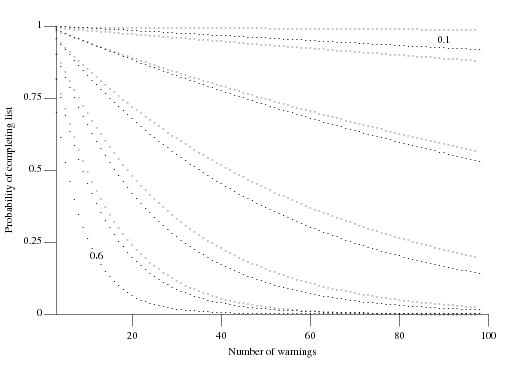

   

   which plots the probability of not encountering a sequence of N consecutive false positive warnings (dots N=3, crosses N=4) after having processed a given number of warning messages for various underlying rates of false positive (ranging from 0.6 to 0.1 in increments of 0.1).

These models are both based on the false positive rate as judged by the developer, which need not reflect reality. For instance, when dealing with warnings involving complex constructs a developer may be unwilling to put the effort into understanding what is going on and either go along with the what the static analysis tool says, thus underestimating the actual false positive rate, or default to assuming the waring is a false positive, thus overestimating the actual false positive rate.

I have been meaning to write about this topic for a while and an email from Paul Anderson galvanized me into action. Paul’s email involved a slightly different issue “… if the human has seen lots of false positives, there is an increased probability that a true positive will be misjudged as a false positive.”

In some companies developers are required to process each message generated by a tool. Now if a developer looses confidence in a tool it would look suspicious if at some point they simply flagged all subsequent warnings as false positives. What algorithm might such developers use to ‘recalibrate’, e.g., skipping over the next M warnings? This sounds like a problem in foraging theory and a possible topic for a future post.

Four years ago I started work as an adviser to the Monitoring Trustee appointed by the European Commission in the EU/Microsoft competition court case. The work revolved around the protocol specification documents being written by Microsoft; at the time these documents were super secret but they are now publicly available for download.

The EU case involved the server protocols, known as WSPP, (the US/Microsoft case involved the client protocols) and with so many of them, over 100, attempts were made to divide them into distinct subsets for licensing to third parties who might only be interested in specific functionality.

On starting one of the first things I did was to create a graph like the one below (this one was created by extracting document cross reference information, using PowerGREP, from the public specifications and plotting it using Graphviz). Each line in the plot represents a dependency between the two protocols whose name’s appear in the ellipsoid nodes (actually a cross reference link in the normative sections of one protocol document to another protocol document).

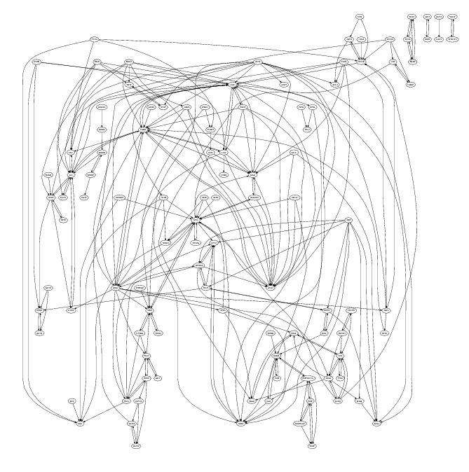
To simplify the diagram references to the ten most referenced protocol documents (i.e., MS-RPCE, MS-ADTS, MS-SMB, MS-KILE, MS-NLMP, MS-SPNG, MS-NRPC, MS-DRSR, MS-DCOM and MS-ADSC) have been excluded. The fact that these protocols are so pervasive is a good indicator of their core importance.

I was not surprised when I saw this graph. When new protocols were added to WSPP it would make sense for developers to make use of functionality provided by existing protocols, creating a dependency.

This extent of the dependencies between these protocol creates advantages and disadvantages for Microsoft. One advantage is that a potential competitor has to make a huge investment in implementing everything (so huge I don’t expect anybody will do it; Samba are nibbling away on a tiny corner); it does not look like its possible to focus on just the most profitable ones. One disadvantage is that these dependencies will make it very difficult for Microsoft to make substantive changes to their protocols.

Do other collections of networking protocols have similar amounts of dependencies between protocols? I don’t know of any analysis that attempts to answer this question. One problem with analyzing the so called ‘open’ protocols like the RFCs is that the quality of the documentation is not that good, with developers often relying on the source code of existing implementations to fill in any missing details.