Archive
Modeling program LOC growth with recurrence equations
Models predicting the growth, in lines of code, of a program are based on the assumption that future growth follows the same pattern of behavior as past growth. One such model is the recurrence relation:
 , where:
  is LOC at time
  ,
,  is the LOC carried over from release
  , and
, and  is the LOC added after release
  .
.
The solution to this recurrence relation is:  , where:
  is the LOC at time
  .
.
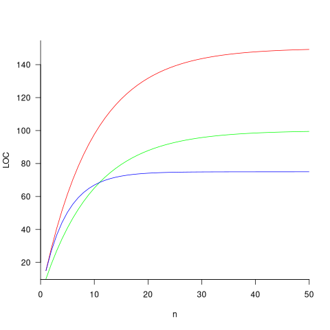
The plot below shows the growth predicted by this model, for various values of  and
and  (code+data):
How close is the fit between this model and actual project growth? The plot below shows the growth in LOC for FreeBSD between 1993 and 2006, data from Herraiz; the red line shows the above equation fitted using non-linear regression, with the blue line showing a fitted linear regression model of the form  (code+data):
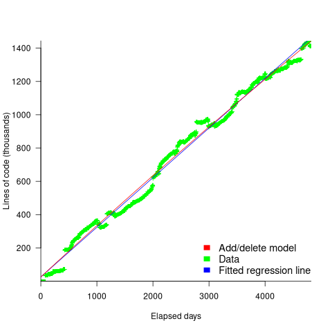
Plugging the fitted coefficients into the recurrence equation when  gives a prediction for the final maximum LOC in FreeBSD of:

The FreeBSD growth is unusual in not having a slow start to its growth, or rather no data is available prior to 1993.
Long-lived, successful projects usually attract new developers, and over time some developers leave. The size of a project, and the predispositions of those involved, can limit the number of active core developers. The above model can be applied to the growth in the number of active developers, i.e.,
 , where:
  is active developers at time
  ,
,  is the developers ceasing to be active
  , and
, and  is the number of new active developers at
  . The solution is:

Adding the developer growth equation in to the LOC model, we get:
 , where
  is now multiplied by the number of developers at time
  , i.e.,
  . The solution to these recurrence equations is somewhat involved (note: if you are using an LLM to check the answers, ChatGPT makes multiple mistakes, but the Grok response contains just one algebra mistake); when
  the equation is:

Checking this more complicated model against another project, the plot below shows the growth of the GNU C library between 1990 and 2011, data from Gonzalez-Barahona, Robles, Herraiz and Ortega; the red line is the fitted equation  (code+data):
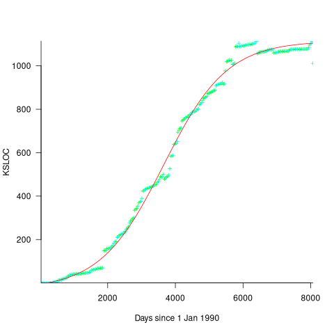
Unsurprisingly, I was not able to fit the more complicated growth model, using non-linear least squares, to the glibc LOC data. The problem was not being able to mimic the slow initial growth rate. I suspect that the developer growth model might be just wrong. Development work on a project does not last forever, and the number of developers will start decreasing at some point. For large projects, the Rayleigh distribution has been found to approximate staffing levels.
Data on project developer numbers over time is rare. The Linux kernel data shows an exponential developer growth rate, but I suspect that this is mostly caused by many one-time only developer contributing towards a new device driver (which are responsible for much of the Kernel growth).
Discussing new language features is more fun than measuring feature usage in code
How often are the features supported by a programming language used by developers in the code that they write?
This fundamental question is rarely asked, let alone answered (my contribution).
Existing code is what developers spend their time reading, compilers translating to machine code, and LLMs use as training data.
Frequently used language features are of interest to writers of code optimizers, who want to know where to focus their limited resources (at least I did when I was involved in the optimization business; I was always surprised by others working in the field having almost no interest in measuring user’s code), and educators ought to be interested in teaching what students are mostly likely to be using (rather than teaching the features that are fun to talk about).
The unused, or rarely used language features are also of interest. Is the feature rarely used because developers have no use for the feature, or does its semantics prevent it being practically applied, or some other reason?
Language designers write books, papers, and blog posts discussing their envisaged developer usage of each feature, and how their mental model of the language ties everything together to create a unifying whole; measurements of actual source code very rarely get discussed. Two very interesting reads in this genre are Stroustrup’s The Design and Evolution of C++ and Thriving in a Crowded and Changing World: C++ 2006–2020.
Languages with an active user base are often updated to support new features. The ISO C++ committee is aims to release a new standard every three years, Java is now on a six-month release cycle, and Python has an annual release cycle. The primary incentives driving the work needed to create these updates appears to be:
- sales & marketing: saturation exposure to adverts proclaiming modernity has warped developer perception of programming languages, driving young developers to want to be associated with those perceived as modern. Companies need to hire inexperienced developers (who are likely still running on the modernity treadmill), and appearing out of date can discourage developers from applying for a job,
- designer hedonism and fuel for the trainer/consultant gravy train: people create new programming languages because it’s something they enjoy doing; some even leave their jobs to work on their language full-time. New language features provides material to talk about and income opportunities for trainers/consultants.
Note: I’m not saying that adding new features to a language is bad, but that at the moment worthwhile practical use to developers is a marketing claim rather than an evidence-based calculation.
Those proposing new language features can rightly point out that measuring language usage is a complicated process, and that it takes time for new features to diffuse into developers’ repertoire. Also, studying source code measurement data is not something that appeals to many people.
Also, the primary intended audience for some language features is library implementors, e.g., templates.
There have been some studies of language feature usage. Lambda expressions are a popular research subject, having been added as a new feature to many languages, e.g., C++, Java, and Python. A few papers have studied language usage in specific contexts, e.g., C++ new feature usage in KDE.
The number of language features invariably grow and grow. Sometimes notice is given that a feature will be removed from a future reversion of the language. Notice of feature deprecation invariably leads to developer pushback by the subset of the community that relies on that feature (measuring usage would help prevent embarrassing walk backs).
If the majority of newly written code does end up being created by developers prompting LLMs, then new language features are unlikely ever to be used. Without sufficient training data, which comes from developers writing code using the new features, LLMs are unlikely to respond with code containing new features.
I am not expecting the current incentive structure to change.
Number of statement sequences possible using N if-statements
I recently read a post by Terence Tao describing how he experimented with using ChatGPT to solve a challenging mathematical problem. A few of my posts contain mathematical problems I could not solve; I assumed that solving them was beyond my maths pay grade. Perhaps ChatGPT could help me solve some of them.
To my surprise, a solution was found to the first problem I tried.
I simplified the original problem (involving Motzkin numbers, details below) down to something that was easier for me to explain to ChatGPT. Based on ChatGPT’s response, it appeared lost, so I asked what it knew about Motzkin numbers. I then reframed the question around the concepts in its response, and got a response that, while reasonable, was not a solution. My question was not precise enough, and a couple of question/answer iterations later, ChatGPT broke the problem down into a series of steps that I saw could solve the problem. While the equation it used in its answer was just wrong, I knew what the correct equation was. So while ChatGPT frequently went off in the wrong direction and got its maths wrong, it helped me refine my statement of the problem and ChatGPT eventually gave steps to a solution which were blindingly obvious to me when I read them.
The question I wanted to answer was: How many distinct statement sequences can be created using 
if-statements and  simple-statements (for a total of
  statements)?
A simple-statement might be an assignment or function call, but not any kind of compound statement, such as a loop. Three sequences are possible using one if-statement and two simple-statements. The if-statement occupies two lines, i.e., the condition and termination curly-bracket, }, as follows:
s1; if (c1) { if (c1) { if (c1) { s1; s1; s2; s2; } } } s2; |
In a previous post I showed how a variant of this question, involving any number of if-statements, can be mapped to a combinatorial interpretation of Motzkin numbers and treating matching up/down diagonals along a path as an if-statement.
ChatGPT performed poorly when I phrased the problem in combinatorial terms (or perhaps my phrasing was poor), so I switched to using a lattice path approach. I asked: “How many lattice paths of length S containing exactly N occurrences of the step (1, 1) and N occurrences of the step (1, -1) are possible?”, and after reading the response I replied “Your analysis does not take into account the fact that the path cannot go below the x-axis. Rework your analysis to take this restriction into account.”
The following is my edited version of ChatGPT’s ‘solution’ response:
“Problem Restated:
We need to count the number of valid Dyck paths of length  , where the path consists of:
Exactly  upward steps (1,1).
Exactly  downward steps (1,−1).
The remaining steps (which must be  horizontal steps (1,0)).
These paths must never dip below the x-axis, and they must return to the x-axis at the end.
…
Step 2: Catalan Numbers for Balanced Paths
If we ignore the horizontal steps for the moment, the number of ways to place  upward steps and
  downward steps such that the path does not go below the x-axis is given by the Catalan number
  :
:

This Catalan number counts the number of valid ways to arrange the  upward steps and
  downward steps such that the path remains above or on the x-axis.
Step 3: Placing Horizontal Steps
Once the valid upward and downward steps have been arranged in a Catalan structure, we can freely place the  horizontal steps (1,0) in the remaining positions of the path. Since there are
  steps (upward and downward) and
  horizontal steps, there are
  gaps (before, after, or between the upward/downward steps) where the horizontal steps can be placed.
The number of ways to place  horizontal steps in these
  positions is given by a binomial coefficient:”
For some reason, ChatGPT gives the wrong binomial coefficient. Calculating the number of ways of distributing  items into
  bins is a well known problem; when a bin can contain zero items, the solution is:
  .
.
Combining the equations from the two steps gives the number of distinct statement sequences that can be created using 
if-statements and  simple-statements as:

The above answer is technically correct, however, it fails to take into account that in practice an if-statement body will always contain either another if-statement or a simple statement, i.e., the innermost if-statement of any nested sequence cannot be empty (the equation used for distributing items into bins assumes a bin can be empty).
Rather than distributing  statements into
  gaps, we first need to insert one simple statement into each of the innermost if-statements. The number of ways of distributing the remaining statements are then counted as previously. How many innermost if-statements can be created using
  if-statements? I found the answer to this question in a StackExchange question, using traditional search.
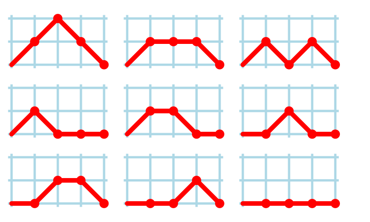
The question can be phrased in terms of peaks in Dyck paths, and the answer is contained in the Narayana numbers (which I had never heard of before). The following example, from Wikipedia, shows the number of paths containing a given number of peaks, that can be produced by four if-statements:
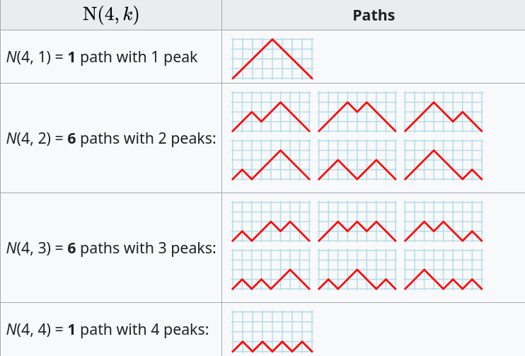
The sum of all these paths is the Catalan number for the given number of if-statements, e.g., using  to denote the Narayana number:
  .
.
Adding at least one simple statement to each innermost if-statement changes the equation for the number of statement sequences from  , to:
, to:

The following table shows the number of distinct statement sequences for five-to-twenty statements containing one-to-five if-statements:
                   N if-statements
           1       2       3       4       5
   5       6       1
   6      10       6
   7      15      20       1
   8      21      50       7
   9      28     105      29       1
  10      36     196      91       9
  11      45     336     238      45       1
  12      55     540     549     166      11
S 13      66     825   1,155     504      66
  14      78   1,210   2,262   1,332     286
  15      91   1,716   4,179   3,168   1,002
  16     105   2,366   7,351   6,930   3,014
  17     120   3,185  12,397  14,157   8,074
  18     136   4,200  20,153  27,313  19,734
  19     153   5,440  31,720  50,193  44,759
20 171 6,936 48,517 88,458 95,381 |
The following is an R implementation of the calculation:
Narayana=function(n, k) choose(n, k)*choose(n, k-1)/n

Catalan=function(n) choose(2*n, n)/(n+1)


if_stmt_possible=function(S, N)
{
return(Catalan(N)*choose(S, 2*N)) # allow empty innermost if-statement
}


if_stmt_cnt=function(S, N)
{
if (S <= 2*N)
   return(0)
total=0
for (k in 1:N)
   {
   P=Narayana(N, k)
   if (S-P*k >= 2*N)
      total=total+P*choose(S-P*k, 2*N)
   }

return(total)
}

isc=matrix(nrow=25, ncol=5)

for (S in 5:20)
   for (N in 1:5)
      isc[S, N]=if_stmt_cnt(S, N)

print(isc) |
Measuring non-determinism in the Linux kernel
Developers often assume that it’s possible to predict the execution path a program will take, for a given set of input values, i.e., program behavior is deterministic. The execution path may be very complicated, and may depend on the contents of certain files (e.g., SQL engines), but it’s deterministic.
There is one kind of program where determinism is not an option; operating systems are non-deterministic when running in a mode where interrupts can occur.
How much non-determinism can occur in, say, Linux? For instance, when a program calls a system function (e.g., open, read, write, close), how often does the execution sequence follow the function call tree that appears in the source code, and how many different call sequences actually occur during program execution (because of diversions caused by an interrupt; ignoring control flow within functions)?
A study by Imanol Allende ran the same program 500K+ times, and traced every function call that occurred within the Linux kernel (thanks to Imanol for sending me the data and answering my questions). The program used appears below; the system calls traced were open (two distinct calls), read, write, and close (two distinct calls); a total of six system calls.
// #includes omitted int main(int argc, char **argv) { unsigned char result; int fd1, fd2, ret; char res_str[10]={0}; fd1 = open("/dev/urandom", O_RDONLY); fd2 = open("/dev/null", O_WRONLY); ret = read(fd1 , &result, 1); sprintf(res_str ,"%d", result); ret = write(fd2, res_str, strlen(res_str)); close(fd1); close(fd2); return ret; } |
Analysing each of these six distinct calls, in around 98% of program runs, each call follows the same sequence of function calls within the kernel (the common case for write involves a chain of around 10 function calls). During the other 2’ish% of calls, the common sequence was interrupted for some reason, and the logged call trace includes additional called functions, e.g., calls involving the Read, Copy, Update synchronization mechanism. The plot below shows the growth in the number of unique traces against the number of program runs (436,827 of them) for the close(fd2) call; a fitted regression line is in red, with the first 1,000 runs not included in the fit (code+data):
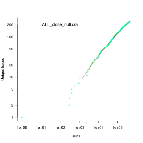
The fitted regression model is  , suggesting that the growth in unique traces is slowing (this equation peaks at around
  ), while the model fitted to some of the system calls implies ever continuing growth.
Allende investigated more sophisticated techniques for estimating the total number of unique traces, including: extreme value theory and species estimation techniques from ecology.
While around 98% of traces are the common case, over half of the unique traces occurred once in 436,827 runs. The plot below shows the number of occurrences of each unique trace, for the close(fd2) call, with an attempted fit of a bi-exponential model (in red; code+data):
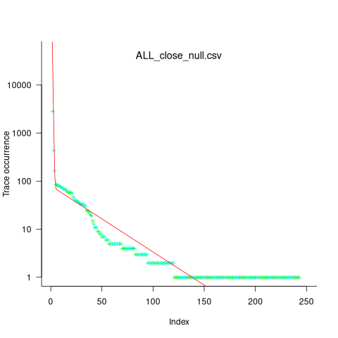
The analysis above looked at one system call, the program contains six system calls. If, for each system call, the probability of the most common trace is 98%, then the probability of all six calls following their respective common case is 89%. As the number of distinct system calls made by a program goes up, the global common case becomes less common, and the number of distinct program traces increases multiplicatively.
Survival of CVEs in the Linux kernel
Software contained in safety related applications has to have a very low probability of failure.
How is a failure rate for software calculated?
The people who calculate these probabilities, or at least claim that some program has a suitably low probability, don’t publish the details or make their data publicly available.
People have been talking about using Linux in safety critical applications for over a decade (multiple safety levels are available to choose from). Estimating a reliability for the Linux kernel is a huge undertaking. This post is taking a first step via a broad brush analysis of a reliability associated dataset.
Public fault report logs are a very messy data source that needs a lot of cleaning; they don’t just contain problems caused by coding mistakes, around 50% are requests for enhancement (and then there is the issue of multiple reports having the same root cause).
CVE number are a curated collection of a particular kind of fault, i.e., information-security vulnerabilities. Data on 2,860 kernel CVEs is available. The data includes the first released version of the kernel containing the problem, and the version of the fixed release. The plot below shows the survival curve for kernel CVEs, with confidence intervals in blue/green (code+data):
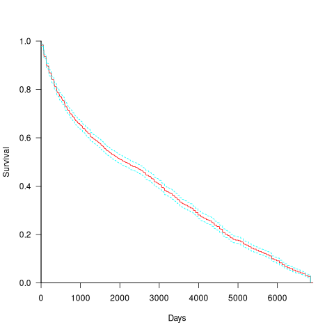
The survival curve appears to have two parts: the steeper decline during the first 1,000 days, followed by a slower, constant decline out to 16+ years.
Some good news is that many of these CVEs are likely to be in components that would not be installed in a safety critical application.
Recent Comments