Sampling error in software engineering
In the physical sciences, measurement error occurs because of accuracy limits on the device used to make the measurement and the interpretation of the data by the person doing the measurement.
In software engineering, some measurements appear to be error free. For instance, lines of code is a discrete value that is easily counted. While some people don’t include blank lines and/or comments, the choice of what to count does not prevent an exact count being made.
In physics, the behavior of particular elements does not depend on the identity of which atoms are measured, while in software the behavior of programs written to the same specification can have different characteristics, e.g., lines of code.
For instance, each implementation of the 3n+1 problem will contain some number of LOC, with other implementations often containing a different number of LOC. The plot below shows the distribution of LOC for 6,301 implementations of 3n+1 (code and data):

Each program implementing the 3n+1 problem is one sample from the population of programs implementing the 3n+1 specification. Different people are likely to implement different programs, and the same person may create different implementations at different times.
Sampling error occurs when the characteristics of a sample are used to infer characteristics about the population from which the sample was drawn.
How might sampling error affect the results of data analysis?
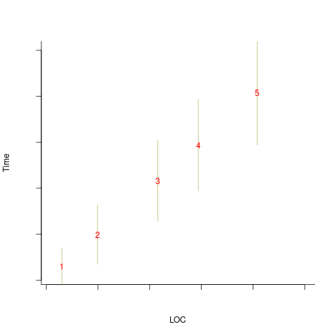
An example, using made-up values: Assume that two sets of sample measurements are made of the time taken to implement five different specifications, along with the lines of code contained in the implementations (in the same language). In the plot below, the yellow circles show a range of likely implementation measurements for each of the five specifications. The green dots, one for each specification, are measurements of one sample of programs implementing each specification; the blue dots are a second sample of programs (code):

The green and blue lines show the ordinary least squares regression model fitted to each sample. The different samples selected from the five populations has produced what appears to be slightly different models. How significant is this difference in the fitted models?
The grey line denotes where LOC is proportional to implementation time, which is one hypothesis of software project progress. The green line sample implies that LOC growth decreases as implementation time increases, while the blue line sample implies the reverse (both have been proposed as hypotheses of software project progress).
The difference in this example is important because the models fitted to the samples straddle the demarcation line between alternative theories of software project development.
A larger sample may not produce a more accurate model; a previous post analyses such a case. The example above shows a symmetric uniformly distributed population because that is the easiest to plot. In practice, populations distributions are likely to be asymmetric and irregular, e.g., measured time may be rounded to the nearest appropriate unit.
The mathematics underpinning OLS assumes that there is no error in the explanatory variables (LOC in the above plot), and that all the error is concentrated in the response variable (Time in the above plot). When there is a non-trivial sample error, or measurement error, OLS is not the appropriate technique to use to fit a regression model. The plot below shows the sample error that is assumed by OLS (code):
When there is a non-trivial error in the explanatory variable (LOC in this example), the appropriate technique for fitting a regression model is errors-in-variables regression.
Building an errors-in-variables regression model requires values for the error in the variables appearing in the equation to be fitted. Obtaining these values can be very difficult (Deming regression is a fitting technique based on the ratio of the errors).
In the above example, what is the likely variability in the implementation time and LOC, for a given specification? The limited data on the LOC contained in multiple implementations of the same specification suggests that the standard deviation of the LOC across implementations of the same specification is around 25% of the mean.
Learning researchers have run experiments where each subject performs the same task multiple times. Performance improves with practice, which makes it difficult to calculate the likely variability in the first-time performance.
My book: Evidence-based software engineering recommends using SIMEX to fit errors-in-variables models (section 11.2.3). This technique takes a model fitted using existing methods (allowing a wide range of models to be fitted), and then refits the model created based on the estimated error in one or more explanatory variables (no need to estimate an error in the response variable, the technique makes use of the value from the initial fit).
Recent Comments