The Shape of Code

The paper Empirically Testing Predictions of an Attrition on Warfare Model for the War in Ukraine, by Peter Turchin, recently showed up during one of my regular searches for software engineering data. A quick scan of the paper founded that it is very empirical, and that the analysis coding was done in R; I could not resist checking out the source code.

One of my first jobs was helping academics fix coding issues with the programs they had written to solve scientific/engineering problems, and this R code reminded me of several habits of scientists who code: the single letter variables used in equations are directly mapped to identifier names, and there is no structure to the code. The code is so short (86 lines) that the lack of structure is a minor inconvenience; a few thousand lines, and it becomes a major headache. The code for Imperial’s COVID model was ten times larger.

Two mistakes in the code/paper jumped out at me, leading to this post. First, some background.

The empirical predictions in the paper are intended to provide insight into who is likely to win the ongoing Ukraine/Russia war. Fighting requires soldiers and these are killed/wounded over time. The country that does not have enough soldiers to at least keep the opposition at bay, looses.

Turchin has proposed what he calls the Attrition War model, based on Lanchester’s laws (various attempts to validate Lanchester’s models, lots of maths to shake a stick at), and the paper solves this model’s set of eight differential equations (each country has the same set of four equations; the connection between the two sets is that one country’s casualty rate and Army size is influenced by the opposing country’s stock of war matériel). The four quantities modelled are casualties, army size, stock of warfare matériel, and production capacity.

Getting predictions out of differential equations requires being able to find a solution to the equations and feeding in numeric values for the various parameters.

Solving the equations is a maths problem, i.e., no knowledge of military matters required. Selecting the equations to solve and the numeric values to feed into the solution is what requires military knowledge. I don’t know anything about military matters; the following analysis is purely related to writing code to solve a set of differential equations, using the equations plus numeric values in Turchin’s November 2023 paper.

For obvious reasons, countries involved in the war do not publish information on the quantities modelled by these equations (which are also likely to be time-dependent). Turchin addresses the changeable nature of the numeric values by introducing various random components into his Attrition model.

From the perspective of solving the eight equations and presenting the results, the following are the two mistakes that jumped out at me (both involving the implementation of the random component):

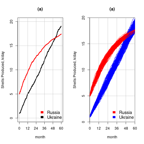
• When a model contains a random component, there will be a huge/infinite number of possible solutions. The takeaway plots in the paper show a single solution (for each of the four variables/two countries), with the width of the plotted lines and their fluctuating appearance suggesting that they contain multiple solutions. The plot below left shows the solution for artillery shell production over time, as it appears in the paper, while the plot below right shows 100 solutions (each line is a different solution; code):

  

  The wedge of lines shows the range of possible solutions (each line drawn overwrites anything previously drawn, and plotting with transparent colors would show the density of solution at a given point; I decided to keep the code simple).

• All the random components are assumed to have a Gaussian distribution. When distribution information is not available, this is usually a safe choice. However, two of the random components must always have non-negative values (i.e., casualties and matériel used can never be negative). The Poisson distribution is the obvious candidate, and a simple search turned up an empirical paper agreeing with this choice (at least for casualties).

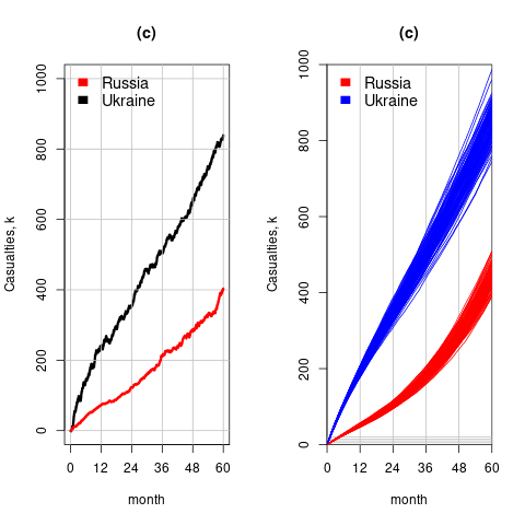
  The plot below left shows one solution for the number of casualties over time, using the original code, while the plot below right shows 100 solutions using a Poisson distribution for the random component (code):

  

  With a Poisson random component, the solutions don’t meander as much, and the variance is smaller than when a Gaussian is used. Technically, it is a more accurate model (if more variance is to be expected a Negative Binomial distribution could be used; see commented out code)

  The latest (November) UK government estimate of Russian casualties is 300K, roughly three times larger than predicted by Turchin’s model. Changing the value for the ‘conversion rate of expended matériel to casualties’ from to brings the casualty prediction inline with current estimates (we have been hearing a lot about the accuracy of the Ukrainian targetting; see code for details).

I have also reworked the code to add some structure, e.g., separating out solving the equations and setting the initial conditions.

Turchin used the traditional approach to solving differential equations, the one we are taught at school. Before seeing the code, I was half expecting to see a System dynamics approach. The advantage of a systems dynamic approach is flexibility (i.e., easier to add more components) and visualization (i.e., a chart showing what feeds into/out of what); an example. There is an R-based book: System Dynamics Modelling with R.