Archive
Relative performance of computers since the 1990s
What was the range of performance of desktop’ish computers introduced since the 1990s, and what was the annual rate of performance increase (answers for earlier computers)?
Microcomputers based on Intel’s x86 family was decimating most non-niche cpu families by the early 1990s. During this cpu transition a shift to a new benchmark suite followed a few years behind. The SPEC cpu benchmark originated in 1989, followed by a 1992 update, with the 1995 update becoming widely used. Pre-1995 results don’t appear on the SPEC website: “Because SPEC’s processes were paper-based and not electronic back when SPEC CPU 92 was the current benchmark, SPEC does not have any electronic storage of these benchmark results.” Thanks to various groups, some SPEC89/92 results are still available.
The following analysis uses the results from the SPEC integer benchmarks, which was changed in 1992, 1995, 2000, 2008, and 2017.
Every time a benchmark is changed, the reported results for the same computer change, perhaps by a lot. The plot below shows the results for each version of the benchmark (code+data):

Provide a few conditions are met, it is possible to normalise each set of results, allowing comparisons to be made across benchmark changes. First, results from running, say, both SPEC92 and SPEC95 on some set of computer needs to be available. These paired results can be used to build a model that maps result values from one benchmark to the other. The accuracy of the mapping will depend on there being a consistent pattern of change, i.e., a strong correlation between benchmark results.
The plot below shows the normalised results, along with regression models fitted to each release (code+data):

What happened around 2007? Dennard scaling stopped, and there is an obvious meeting of two curves as one epoch transitioned into another. Since 2007 performance improvements have been driven by faster memory, larger caches, and for some applications multiple on-die cpus.
The table below shows the annual growth in SPECint performance for each of the benchmark start years, over their lifetime.
      Year   Annual growth
      1992       26.2%
      1995       25.9%
      2000       14.2%
      2007       13.9%
2017 10.5% |
In 2025, the cpu integer performance of the average desktop system is over 100 times faster than the average 1992 desktop system. With the first factor of 10 improvement in the first 10 years, and the second factor of 10 in the previous 20 years.
CPU frequency not relevant to SPEC benchmark performance
Despite the end of Dennard scaling around 2005-7 computer performance, as measured by the SPEC cpu benchmarks, continues to improve. What is driving this ongoing increase in performance, given that cpu clock rates have stopped increasing?
The plot below shows 9,161 results from the SPEC CPU integer benchmark, plus the fitted regression line  (code+data):

There is a scattering of benchmark results because manufacturers offer systems having a range of performance.
Possible factors driving the ongoing increases in system performance include increased DRAM-memory bandwidth, and cpu improvements such as larger caches and more accurate branch prediction. While Moore’s law (i.e., rate of growth of the number of transistors on a chip) has slowed down a lot, the number of transistors in a processor chip has continued to increase (many of these transistors have been used to build chips that contain multiple cpu cores).
The SPEC benchmark result data includes a lot of information about the system that ran the benchmarks, including: processor family/model, number of cpu cores, clock frequency, amount of memory installed and its type.
Results from SPEC CPU2017, the current version of the benchmark, are available from the start of 2017 to now. The following analysis uses these results. Results from the SPEC CPU2006 benchmark are also available, and a regression model fitted to the results from the 780 systems that ran both benchmarks, gives the mapping from CPU INT 2006 to CPU INT 2017 as:  .
.
The processor information in the results file usually specifies family name plus model number/name. The model information usually correlates with clock frequency, perhaps cache size, or gpu support; some examples below.
    AMD EPYC 4464P                AMD EPYC 4564P
    AMD Ryzen 9 7950X             AMD Ryzen 7 5800X
    Intel Xeon Platinum 8490H     Intel Xeon Gold 6438N
Intel Xeon E3-1220 v3 Intel Xeon E5-2697 v3 |
The family name is sufficient for an initial analysis. Details of any cache size differences between models can always be included in a later analysis. The following table shows the number of processor x86 based families present in the 2017 INT results (total 9,161):
           AMD EPYC           AMD Ryzen               Intel
               1475                   7                   1
      Intel Celeron       Intel Core i3       Intel Core i5
                 16                  31                   2
      Intel Core i7       Intel Pentium          Intel Xeon
                  1                  30                 605
  Intel Xeon Bronze        Intel Xeon D       Intel Xeon E3
                167                  12                  16
      Intel Xeon E5       Intel Xeon E7     Intel Xeon Gold
                  3                   2                3994
Intel Xeon Platinum   Intel Xeon Silver        Intel Xeon W
1822 969 8 |
The memory information usually includes total bytes, number of memory sticks and interface standard (e.g., DDR2/3/4/5); some examples below.
    64 GB (2 x 32 GB 2Rx4 PC5-5600B-R, running at 5200)
    64 GB (2 x 32 GB 2Rx8 PC4-3200AA-E)
    256 GB (8*1GB DDR2-400 DIMMS per 4 core module)
    192 GB (4 x 12 x 4 GB DDR3-1333R, ECC, CL9)
    32 GB (8 x 4 GB Dual-rank PC2-6400 CL5-5-5 FB-DIMMs)
24 GB (6 x 4 GB DDR3-1333 downclocked to 1066 MHz) |
The memory bandwidth can be calculated from the interface standard used. The names of modern DRAM interface standards start with either DDR or PC, and a number, a hyphen and then another number. The values appearing in the SPEC results don’t always follow the naming rules listed in the standard (e.g., last number of a PC name using the corresponding DDR number), and in a few cases a digit was dropped from the last number. Where possible the ‘obvious’ edits were made (sometimes values were just wrong), see code for details. The following table shows the number of interface standards represented in the 2017 CPU INT results (total 9,161; in the 2006 results DDR names predominated):
PC4-2400  PC4-2666  PC4-2933  PC4-3200  PC4-4800 PC5-11200 PC5-12800
      26      2248      2163      2080         6         2         3
PC5-4800  PC5-5200  PC5-5600  PC5-6400     PC5-8  PC5-8800
1735 5 653 233 2 5 |
Once the memory is identified, its bandwidth can be looked up (bespoke memory stick clock rates were ignored). Fitting a regression model to the data, with the CPU INT (cpu integer benchmark) result as the outcome, we get (using a multiplicative model allows each factor to have a percentage impact; code+data):

where:  is the memory bandwidth in megabytes per second,
  is cpu frequency in MHz, and
  is the fitted constant for each processor family.
The cpu frequency varies between 1.7 and 4.7 GHz (a ratio of 1:2.8), the memory bandwidth between 19,200 and 51,200 MB/s (a ratio of 1:2.7), and processor family performance impact ratio was 1:2.2. Given the fitted power laws, this range of cpu frequencies could impact performance by around 22%, while the range of memory bandwidth could impact performance by a factor of two.
This fitted model implies that cpu frequency changes, over the range supported by systems since 2017, have almost no impact on the performance of integer-based programs, i.e., no floating point.
I thought there might be a correlation between memory bandwidth and cpu frequency (because vendors would use faster memory in systems with faster cpus). The plot below shows CPU frequency against memory bandwidth (both axis use linear scales), plus a fitted regression line in red (code+data):
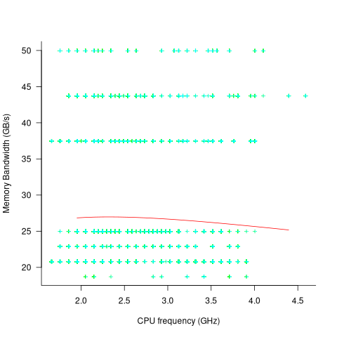
I was wrong. There does not appear to be any connection between a system’s cpu frequency and its memory bandwidth.
These days, most x86 chips include multiple processors, with each processor taking a share of memory bandwidth. Increasing memory bandwidth is essential, if all cores are to be kept busy.
The SPEC CPU benchmark measures the performance of a single processor. If only one of the cpu cores available on a system is being used, that core has the benefit of memory bandwidth that usually has to be shared.
To what extent is a single core benchmark relevant today? I suspect that most programs run on a single core, but developers sometimes attempt to spread cpu intensive programs over multiple cores. As always, data is needed.
The SPEC benchmark is useful for cpu designers (the original target market) and compiler writers wanting to measure the impact of fancy new optimizations.
Memory capacity growth: a major contributor to the success of computers
The growth in memory capacity is the unsung hero of the computer revolution. Intel’s multi-decade annual billion dollar marketing spend has ensured that cpu clock frequency dominates our attention (a lot of people don’t know that memory is available at different frequencies, and this can have a larger impact on performance that cpu frequency).
In many ways memory capacity is more important than clock frequency: a program won’t run unless enough memory is available but people can wait for a slow cpu.
The growth in memory capacity of customer computers changed the structure of the software business.
When memory capacity was limited by a 16-bit address space (i.e., 64k), commercially saleable applications could be created by one or two very capable developers working flat out for a year. There was no point hiring a large team, because the resulting application would be too large to run on a typical customer computer. Very large applications were written, but these were bespoke systems consisting of many small programs that ran one after the other.
Once the memory capacity of a typical customer computer started to regularly increase it became practical, and eventually necessary, to create and sell applications offering ever more functionality. A successful application written by one developer became rarer and rarer.
Microsoft Windows is the poster child application that grew in complexity as computer memory capacity grew. Microsoft’s MS-DOS had lots of potential competitors because it was small (it was created in an era when 64k was a lot of memory). In the 1990s the increasing memory capacity enabled Microsoft to create a moat around their products, by offering an increasingly wide variety of functionality that required a large team of developers to build and then support.
GCC’s rise to dominance was possible for the same reason as Microsoft Windows. In the late 1980s gcc was just another one-man compiler project, others could not make significant contributions because the resulting compiler would not run on a typical developer computer. Once memory capacity took off, it was possible for gcc to grow from the contributions of many, something that other one-man compilers could not do (without hiring lots of developers).
How fast did the memory capacity of computers owned by potential customers grow?
One source of information is the adverts in Byte (the magazine), lots of pdfs are available, and perhaps one day a student with some time will extract the information.
Wikipedia has plenty of articles detailing cpu performance, e.g., Macintosh models by cpu type (a comparison of Macintosh models does include memory capacity). The impact of Intel’s marketing dollars on the perception of computer systems is a PhD thesis waiting to be written.
The SPEC benchmarks have been around since 1988, recording system memory capacity since 1994, and SPEC make their detailed data public 🙂 Hardware vendors are more likely to submit SPEC results for their high-end systems, than their run-of-the-mill systems. However, if we are looking at rate of growth, rather than absolute memory capacity, the results may be representative of typical customer systems.
The plot below shows memory capacity against date of reported benchmarking (which I assume is close to the date a system first became available). The lines are fitted using quantile regression, with 95% of systems being above the lower line (i.e., these systems all have more memory than those below this line), and 50% are above the upper line (code+data):
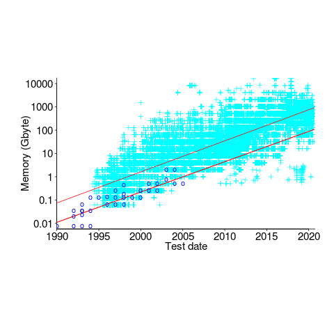
The fitted models show the memory capacity doubling every 845 or 825 days. The blue circles are memory that comes installed with various Macintosh systems, at time of launch (memory doubling time is 730 days).
How did applications’ minimum required memory grow over time? I have a patchy data for a smattering of products, extracted from Wikipedia. Some vendors probably required customers to have a fairly beefy machine, while others went for a wider customer base. Data on the memory requirements of the various versions of products launched in the 1990s is very hard to find. Pointers very welcome.
Honking the horn for go faster memory (over go faster cpus)
I have been doing some analysis of computer performance, as measured by the results of the SPEC 2006 int benchmark (i.e, no floating point). As the following plot shows, computers are continuing to get faster (code and data):
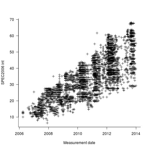
I think the widening spread of results might have a lot to do with companies slowly migrating to the newer benchmark, increasing the range of test cases; there mus also be an element of an increasing range of computer performance on offer from vendors now we have reached the good-enough point.
In the last century the increase in performance was strongly correlated with increasing cpu clock speed. As the following plot shows, this century is different (in years to come the first few years, where this correlation quickly died out, will be treated as a round-off error); performance is more likely to be higher at a higher clock rate, but far from guaranteed:
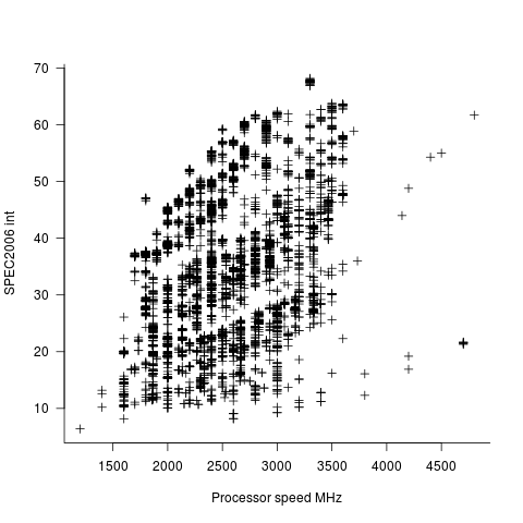
One of the reasons for this change is that, for many tasks, cpus are now seriously performance limited by memory bandwidth, and so these days a lot of the performance improvement is coming from faster memory (yes, it is really about shifting more bytes per clock tick, but a common faster/slower vocabulary keeps things simpler). The following plot uses PC2 (blue) and PC3 (red) module numbers:
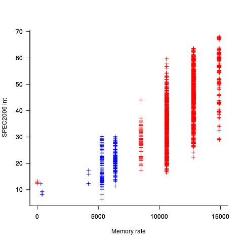
Making use of go faster memory is not as straight-forward as using a go faster cpu. Memory chip configuration includes more tuning options than cpus, which just need a faster clock. That spread in performance, for a given memory rate can probably be traced to use of different options and of course cpu caches play an important part in improving performance. The SPEC results do contain lots of descriptive details about cache characteristics, but extracting it will be fiddly and analysing this kind of stuff always makes my head hurt.
The computer buying public have learned that higher clock rate is better. Unfortunately they still think this applies to cpus when they should now be asking about memory speed. When I ask people about the speed of memory in their computer I am usually told how many gigabytes it has, or get the same kind of look I used to get many years ago when asking about cpu speed.
Changes in optimization performance of gcc over time
The SPEC benchmarks came out a year after the first release of gcc (in fact gcc was and still is one of the programs included in the benchmark). Compiling the SPEC programs using the gcc option -O2 (sometimes -O3) has always been the way to measure gcc performance, but after 25 years does this way of doing things tell us anything useful?
The short answer: No
The longer answer is below as another draft section from my book Empirical software engineering with R book. As always comments welcome.
Changes in optimization performance of gcc over time
The GNU Compiler Collection <book gcc-man_12> (GCC) is under active development with its most well known component, the C compiler gcc, now over 25 years old. After such a long period of development is the quality of code generated by gcc still improving and if so at what rate? The method typically used to measure compiler performance is to compile the [SPEC] benchmarks with a small set of optimization options switched on (e.g., the O2 or O3 options) and this approach is used for the analysis performed here.
Data
Vladimir N. Makarow measured the performance of 9 releases of gcc, occurring between 2003 and 2010, on the same computer using the same benchmark suite (SPEC2000); this data is used in the following analysis.
The data contains the [SPEC number] (i.e., runtime performance) and code size measurements on 12 integer programs (11 in C and one in C+\+) from SPEC2000 compiled with gcc versions 3.2.3, 3.3.6, 3.4.6, 4.0.4, 4.1.2, 4.2.4, 4.3.1, 4.4.0 and 4.5.0 at optimization levels O2 and O3 (the mtune=pentium4 option was also used) 32-bit for the Intel Pentium 4 processor.
The same integer programs and 14 floating-point programs (10 in Fortran and 4 in C) were compiled for 64-bits, again with the O2 and O3 options (the mpc64 floating-point option was also used), using gcc versions 4.0.4, 4.1.2, 4.2.4, 4.3.1, 4.4.0 and 4.5.0.
Is the data believable?
The following are two fitness-for-purpose issues associated with using programs from SPEC2000 for these measurements:
-
the benchmark is designed for measuring processor performance not
compiler performance, -
many of its programs have been used for compiler benchmarking for
many years and it is likely that gcc has already been tuned to do
well on this benchmark.
The runtime performance measurements were obtained by running each programs once, SPEC requires that each program be run three times and the middle one chosen. Multiple measurements of each program would have increased confidence in their accuracy.
Predictions made in advance
Developers continue to make improvements to gcc and it is hoped that its optimization performance is increasing, knowing that performance is at a steady state or decreasing performance is also of interest.
No hypothesis is proposed for how optimization performance, as measured by the O2 and O3 options, might change between releases of gcc over the period 2003 to 2010.
The gcc documentation says that using the O3 option causes more optimizations to be performed than when the O2 option is used and therefore we would expect better performance for programs compiled with O3.
Applicable techniques
Modelling individual O2 and O3 option performance
One technique for modelling changes in optimization performance is to build a linear model that fits the gcc version (i.e., version is the predictor variable) to the average performance of the code it generate, calculating the averaged performance over each of the programs measured with the corresponding version of gcc. The problem with this approach is that by calculating an average it is throwing away information that is available about the variation in performance across different programs.
Building a [mixed-effects] model would make use of all the data when fitting a relationship between two quantities where there is a recurring random component (i.e., the SPEC program used). The optimizations made are likely to vary between different SPEC programs, we could treat the performance variations caused by difference in optimization as being random and having an impact on the mean performance value of all programs.
Programs differ in the magnitude of their SPEC number and code size, the measurements were converted to the percentage change compared against the values obtained using the earliest version of gcc in the measurement set.
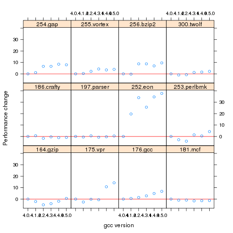
Figure 1. Percentage change in SPEC number (relative to version 4.0.4) for 12 programs compiled using 6 different versions of gcc (compiling to 64-bits with the O3 option).
Fitting a linear model requires at least two sets of [interval data]. The gcc version numbers are [ordinal values] and the following are two possible ways of mapping them to interval values:
-
there have been over 150 different released versions of gcc and a
particular version could be mapped to its place in this sequence. -
the date of release of a version can be mapped to the number of
days since the first release.
If version releases are organized around new functionality added then it makes sense to use version sequence number. If the performance of a new optimization was proportional to the amount of effort (e.g., man days) that went into its implementation then it would make sense to use days between releases.
The versions tested by Makarow were each from a different secondary release within a given primary version line and at roughly yearly intervals (two years separated the first pair and one month another pair).
There have been approximately 25 secondary releases in the 25 year project and using a release version sequence number starting at 20 seems like a reasonable choice.
Internally a compiler optimizer performs many different kinds of optimizations (gcc has over 160 different options for controlling machine independent optimization behavior). While the implementation of a new optimization is a gradual process involving many days of work, from the external user perspective it either exists and does its job when a given optimization level is supported or it does not exist.
What is the shape of the performance/release-version relationship? In the first few years of a compilers development it is to be expected that all the known major (i.e., big impact) optimization will be implemented and thereafter newly added optimizations have a progressively smaller impact on overall performance. Given gcc’s maturity it looks reasonable to assume that new releases contain a few additional improvement that have an incremental impact, i.e., the performance/release-version relationship is assumed to be linear (no other relationship springs out of a plot of the data).
A mixed-effects model can be created by calling the R function lme from the package nlme. The only difference between the following call to lme and a call to lm is the third argument specifying the random component.
t.lme=lme(value ~ variable, data=lme.O2, random = ~ 1 | Name) |
The argument random = ~ 1 | Name specifies that the random component effects the mean value of the result (when building a model this translates to an effect on the value of the intercept of the fitted equation) and that Name (of the program) is the grouped variable.
To specify that the random effect applies to the slope of the equation rather than its intercept the call is as follows:
t.lme=lme(value ~ variable, data=lme.O2, random = ~ variable -1 | Name) |
To specify that both the slope and the intercept are effected the -1 is omitted (for this gcc data the calculation fails to converge when both can be effected).
Since the measurements are about different versions of gcc it is to be expected that the data format has a separate column for each version of gcc (the format that would be used to pass data lm) as follows:
Name v3.2.3 v3.3.6 v3.4.6 v4.0.4 v4.1.2 v4.2.4 v4.3.1 v4.4.0 v4.5.0 1 164.gzip 933 932 957 922 933 939 917 969 955 2 175.vpr 562 561 577 576 586 585 576 589 588 3 176.gcc 1087 1084 1159 1135 1133 1102 1146 1189 1211 |
The relationship between the three variables in the call to lme is more complicated and the data needs to be reorganize so that one column contains all of the values, one the gcc version numbers and another column the program names. The function melt from package reshape2 can be used to restructure the data to look like:
Name variable value 11 256.bzip2 v3.2.3 0.000000 12 300.twolf v3.2.3 0.000000 13 SPECint2000 v3.2.3 0.000000 14 164.gzip v3.3.6 -0.107181 15 175.vpr v3.3.6 -0.177936 16 176.gcc v3.3.6 -0.275989 17 181.mcf v3.3.6 0.148810 |
Comparing O2 and O3 option performance
When comparing two samples the [Wilcoxon signed-rank test] and the [Mann-Whitney U test] spring to mind. However, some of the expected characteristics of the data violate some of the properties that these tests assume hold (e.g., every release include new/updated optimizations which is likely to result in the performance of each release having a different mean and variance).
The difference in performance between the two optimization levels could be treated as a set of values that could be modelled using the same techniques applied above. If the resulting model have a line than ran parallel with the x-axis and was within the appropriate confidence bounds we could claim that there was no measurable difference between the two options.
Results
The following is the output produced by summary for a mixed-effect model, with the random variation assumed to effect the value of intercept, created from the SPEC numbers for the integer programs compiled for 64-bit code at optimization level O2:
Linear mixed-effects model fit by REML
 Data: lme.O2
       AIC      BIC    logLik
  453.4221 462.4161 -222.7111

Random effects:
 Formula: ~1 | Name
        (Intercept) Residual
StdDev:    7.075923 4.358671

Fixed effects: value ~ variable
                 Value Std.Error DF   t-value p-value
(Intercept) -29.746927  7.375398 59 -4.033264   2e-04
variable      1.412632  0.300777 59  4.696612   0e+00
 Correlation:
         (Intr)
variable -0.958

Standardized Within-Group Residuals:
        Min          Q1         Med          Q3         Max
-4.68930170 -0.45549280 -0.03469526  0.31439727  2.45898648

Number of Observations: 72
Number of Groups: 12
|
and the following summary output is from a linear model built from an average of the data used above.
Call:
lm(formula = value ~ variable, data = lmO2)

Residuals:
      13       26       39       52       65       78
 0.16961 -0.32719  0.47820 -0.47819 -0.01751  0.17508

Coefficients:
             Estimate Std. Error t value Pr(>|t|)
(Intercept) -28.29676    2.22483  -12.72 0.000220 ***
variable      1.33939    0.09442   14.19 0.000143 ***
---
Signif. codes:  0 ‘***’ 0.001 ‘**’ 0.01 ‘*’ 0.05 ‘.’ 0.1 ‘ ’ 1

Residual standard error: 0.395 on 4 degrees of freedom
Multiple R-squared: 0.9805,     Adjusted R-squared: 0.9756
F-statistic: 201.2 on 1 and 4 DF,  p-value: 0.0001434
|
The biggest difference is that the fitted values for the Intercept and slope (the column name, variable, gives this value) have a standard error that is 3+ times greater for the mixed-effects model compared to the linear model based on using average values (a similar result is obtained if the mixed-effects random variation is assumed to effect the slope and the calculation fails to converge if the variation is on both intercept and slope). One consequence of building a linear model based on averaged values is that some of the variations present in the data are smoothed out. The mixed-effects model is more accurate in that it takes all variations present in the data into account.
For integer programs compiled for 32-bits there is much less difference between the mixed-effects models and linear models than is seen for 64-bit code.
-
For SPEC performance the created models show:
-
for the integer programs a rate of increase of around 0.6% (sd
0.2) per release forO2andO3options on 32-bit code
and an increase of 1.4% (sd 0.3) for 64-bit code, -
for floating-point, C programs only, a rate of increase per
release of 12% (sd 5) at 32-bits and 1.4% (sd 0.7) at 64-bits, with
very little difference between theO2andO3options.
-
for the integer programs a rate of increase of around 0.6% (sd
-
For size of generated code the created models show:
-
for integer programs 32-bit code built using
O2size is
decreasing at the rate of 0.6% (sd 0.1) per release, while for both
64-bit code andO3the size is increasing at between 0.7% (sd
0.2) and 2.5% (sd 0.4) per release, -
for floating-point, C programs only, 32-bit code built using
O2had an unacceptable p-value, while for both 64-bit code
andO3the size is increasing at between 1.6% (sd 0.3) and
9.3 (sd 1.1) per release.
-
for integer programs 32-bit code built using
Comparing O2 and O3 option performance
The intercept and slope values for the models built for the SPEC integer performance difference had p-values way too large to be of interest (a ballpark estimate of the values would suggest very little performance difference between the two options).
The program size change models showed O3 increasing, relative to O2, at 1.4% to 1.7% per release.
Discussion
The average rate of increase in SPEC number is very low and does not appear to be worth bothering about, possible reasons for this include:
-
a lot of effort has already been invested in making sure that gcc
performs well on the SPEC programs and the optimizations now being
added to gcc are aimed at programs having other kinds of
characteristics, -
gcc is a mature compiler that has implemented all of the worthwhile
optimizations and there are no more major improvements left to be
made, -
measurements based on just setting the
O2orO3
options might not provide a reliable guide to gcc optimization
performance. The command
gcc -c -Q -O2 --help=optimizers
shows that for gcc version 4.5.0 theO2option enables 91 of
the possible 174 optimization options and theO3option
enables 7 more. Performing some optimizations together sometimes
results in poorer quality code than if a subset of those
optimizations had been applied (genetic programming is being
researched as one technique for selecting the best optimizations
options to use for a given program and up to 13% improvements have
been obtained over gcc’s -O options <book Bashkansky_07>). The
percentage performance change figure above shows
that for some programs performance decreases on some releases.Whole program optimization is a major optimization area that has been addressed in recent versions of gcc, this optimizations is not enabled by the
Ooptions.
The percentage differences in SPEC integer performance between the O2 and O3 options were very small, but varied too much to be able to build a reliable linear model from the values.
For SPEC program code size there is a significant different between the O2 and O3 options. This is probably explained by function inlining being one of the seven additional optimization enabled by O3 (inlining multiple calls to the same function often increases code size <book inlining> and changes to the inlining optimization over releases could result in more functions being inlined).
Conclusion
Either the optimizations added to gcc between 2003 and 2010 have not made any significant difference to the performance of the generated code or the established method of measuring gcc optimization performance (i.e., the SPEC benchmarks and the O2 or O3 compiler options) is no longer a reliable indicator.
Recent Comments