Archive
The Norden-Rayleigh model: some history
Since it was created in the 1960s, the Norden-Rayleigh model of large project manpower has consistently outperformed, or close runner-up, other models in benchmarks (a large project is one requiring two or more man-years of effort). The accuracy of the Norden-Rayleigh model comes with a big limitation: a crucial input value to the calculation is the time at which project manpower peaks (which tends to be halfway through a project). The model just does not work for times before the point of maximum manpower.
Who is the customer for a model that predicts total project manpower from around the halfway point? Managers of acquisition contracts looking to evaluate contractor performance.
Not only does the Norden-Rayleigh model make predictions that have a good enough match with reality, there is some (slightly hand wavy) theory behind it. This post delves into Peter Norden’s derivation of the model, and some of the subsequent modifications. Norden work is the result of studies carried out at IBM Development Laboratories between 1956 and 1964, looking for improved methods of estimating and managing hardware development projects; his PhD thesis was published in 1964.
The 1950s/60s was a period of rapid growth, with many major military and civilian systems being built. Lots of models and techniques were created to help plan and organise these projects, two that have survived the test of time are the critical path method and PERT. As project experience and data accumulated, techniques evolved.
Norden’s 1958 paper “Curve Fitting for a Model of Applied Research and Development Scheduling” describes how a project consists of overlapping phases (e.g., feasibility study, deign, implementation, etc), each with their own manpower rates. The equation Norden fitted to cumulative manpower was:  , where
  is project elapsed time,
  is total project manpower, and
  ,
,  , and
, and  are fitted constants. This is the logistic equation with added tunable parameters.
By the early 1960s, Norden had brought together various ideas to create the model he is known for today. For an overview, see his paper (starting on page 217): Project Life Cycle Modelling: Background and Application of the Life Cycle Curves.
The 1961 paper: “The decisions of engineering design” by David Marples was influential in getting people to think about project implementation as a tree-like collection of problems to be solved, with decisions made at the nodes.
The 1958 paper: The exponential distribution and its role in life testing by Benjamin Epstein provides the mathematical ideas used by Norden. The 1950s was the decade when the exponential distribution became established as the default distribution for hardware failure rates (the 1952 paper: An Analysis of Some Failure Data by D.J. Davis supplied the data).
Norden draws a parallel between a ‘shock’ occurring during the operation of a device that causes a failure to occur and a discovery of a new problem to be solved during the implementation of a task. Epstein’s exponential distribution analysis, along with time dependence of failure/new-problem, leads to the Weibull distribution. Available project manpower data consistently fitted a special case of the Weibull distribution, i.e., the Rayleigh distribution (see: Project Life Cycle Modelling: Background and Application of the Life Cycle Curves (starts on page 217).
The Norden-Rayleigh equation is:  , where:
  is work completed,
  is total manpower over the lifespan of the project,
  ,
,  is time of maximum effort per unit time (i.e., the Norden/Rayleigh equation maximum value), and
  is project elapsed time.
Going back to the original general differential equation, before a particular solution is obtained, we have:  , where
  is the amount of work left to do (it’s sometimes referred to as the learning curve). Norden assumed that:
  .
.
The 1980 paper: “An alternative to the Rayleigh curve model for software development effort” by F.N. Parr argues that the assumption of work remaining being linear in time is unrealistic, rather that because of the tree-like nature of problem discovery, the work still be to done,  , is proportional to the work already done, i.e.,
  , leading to:
  , where:
  is some fitted constant.
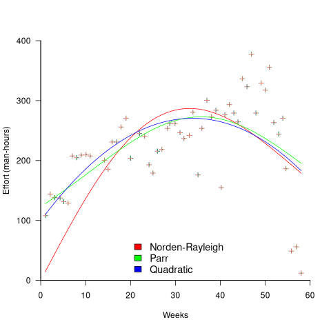
While the Norden-Rayleigh equation looks very different from the Parr equation, they both do a reasonable job of fitting manpower data. The following plot fits both equation to manpower data from a paper by Basili and Beane (code+data):

A variety of alternative forms for the quantity  have been proposed. An unpublished paper by H.M. Hubey discusses various possibilities.
Some researchers have fitted a selection of equations to manpower data, searching for the one that gives the best fit. The Gamma distribution is sometimes found to provide a better fit to a dataset. The argument for the Gamma distribution is not based on any theory, but purely on the basis of being the best fitting distribution, of those tested.
Putnam’s software equation debunked
The implementation of a project has a lifecycle that starts and finishes with zero people working on it. Between starting and finishing, the number of staff quickly grows to a peak before slowly declining. In a series of very hard to obtain papers during the early 1960s (chapter 5), Peter Norden created a large project staffing model described by the Rayleigh equation. This model was evangelized by Lawrence Putnam in the 1970s, who called it the Norden/Rayleigh model, while others sometimes now call it the Norden/Putnam, Putnam/Rayleigh, or some combination of names; Putnam’s papers can be hard to obtain.
The Norden/Rayleigh equation is: 
where:  is work completed,
  is total manpower over the lifespan of the project,
  ,
,  is time of maximum effort per unit time (i.e., the Norden/Rayleigh equation maximum value, which Putnam calls project development time), and
  is project elapsed time.
Norden’s model is only applicable to large projects (e.g., 2+ man-years), and Putnam points out that the staffing of small projects is usually a square wave, i.e., a number of staff are allocated at the start and this number remains the same until project completion.
As well as evangelizing Norden’s model, Putnam also created his own model; an equation connecting delivered lines of code, total manpower and project duration. The usually cited paper for this work is: “A General Empirical Solution to the Macro Software Sizing and Estimating Problem”, which can sometimes be found as a free download. I had always assumed that people did not take this model seriously, and it was not worth my time debunking it. The paper makes conjures hand-wavy connections between various equations which don’t seem to go anywhere, and eventually connects together a regression equation fitted to nine data points with an observation+assumption about another regression equation to create what Putnam calls the software equation:  , where
  is delivered source code statements, and
  is a constant.
I recently read a 2014 paper by Han Suelmann debunking Putnam’s software equation, which led me to question my assumption about people not using Putnam’s model. Google Scholar shows 1,411 citations, with 133 since 2020. It looks like the software equation is still being taken seriously (or researchers are citing it because everybody else does; a common practice).
Why isn’t Putnam’s software equation worth treating seriously?
First, Putnam’s derivation of the software equation reads like a just-so story based on a tiny amount of data, and second a larger independent dataset does not show the pattern seen in Putnam’s data.
The derivation of the software equation starts by defining productivity as the number of delivered source code statements divided by the total manpower consumed to produce them,  . Ok.
. Ok.
There is more certainty to a line fitted to a set of points that roughly follow a straight line, than to fit a line to points that follow a curve (because there are usually many ‘curve’ equations to choose from). The Norden/Rayleigh equation can be transformed to a form that is amenable to fitting a straight line, i.e., dividing by time and taking logs, as follows (which plugs in the value of  ):
):

Putnam noticed (or perhaps it was the authors of the cited prepublication paper “Software budgeting model” by G. E. P. Box and L. Pallesen, which I cannot locate a copy of) that when plotting  against
  : “If the number
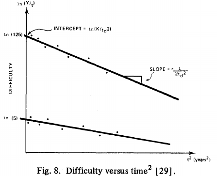
  was small, it corresponded with easy systems; if the number was large, it corresponded with hard systems and appeared to fall in a range between these extremes.” Notice that in the screenshot of a figure from Putnam’s paper below, the y-axis is labelled “Difficulty”, not with the quantity actually plotted.

Based on an observation about easy/hard systems (it is never explained how easy/hard is measured) something called difficulty is defined to be:  . No explanation is given for dropping the log scaling, or the possibility that some other relationship might hold.
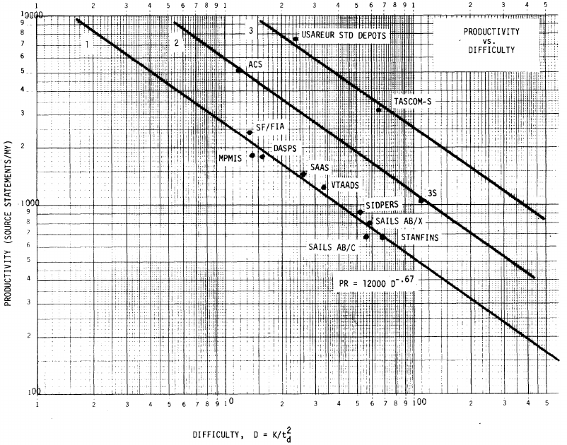
The screenshot below is of a figure from Putnam’s paper, which plots the values of  against
  for 13 projects. The fitted regression lines (the three lines are fitted using, 9, 2 and 2 points of the 13 projects) have the form
  , i.e.,
  (I extracted the points and fitted
  ; code+extracted data):

With a bit of algebra, the two equations:  and
and  , can be combined to create the software equation.
Yes, Putnam’s software equation was hand-waved into existence by plucking a “difficulty” component from an observation about the behavior of projects in a regression model and equating it to a regression line fitted to nine points.
Are the patterns seen by Putnam found in other projects?
In the 1987 paper “Time-Sensitive Cost Models in the Commercial MIS Environment” D. Ross Jeffery used data from 47 projects to investigate the effort/time relationships used by Putnam to derive his software equation.
The plot below, of log(Difficulty) vs log(Productivity), shows what appears to be a random scattering of points, confirmed by failing to fit a regression model (code+extracted data):

No. The patterns seen by Putnam are not present in these projects. I don’t think that the difference in application domain is relevant (Putnam’s projects were for Military systems and Jeffery’s are for commercial projects). Norden’s model is not specific to software projects.
Jeffery’s uses a regression model to find:  , the corresponding Putnam equation is:
  (the paper does not include the plot needed to extract the required data). The
  exponent might be claimed to be close enough, but the
  exponent is very different.
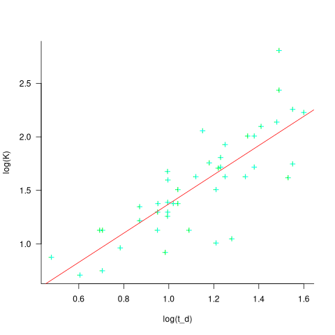
Jeffery’s paper includes a plot of  against
  , and the plot below shows the extracted data (44 points), plus fitted regression line (code+extracted data):

The regression line has the form  . This relationship further undermines assumptions made by Putnam, e.g., smaller systems are easier.
The Han Suelmann paper that triggered this post takes a very different approach to debunking Putnam’s model (he uses simulation to show that random data, drawn from a suitable distribution, can produce the patterns seen by Putnam).
Recent Comments