Archive
Percentage of methods containing no reported faults
It is often said, with some evidence, that 80% of reported faults, for a program, occur in 20% of its code. I think this pattern is a consequence of 20% of the code being executed 80% of the time, while many researchers believe that 20% of the source code has characteristics that result in it containing 80% of the coding mistakes.
The 20% figure is commonly measured as a percentage of methods/functions, rather than a percentage of lines of code.
This post investigates the expected fraction of a program’s methods that remain fault report free, based on two probability models.
Both models assume that coding mistakes are uniformly scattered throughout the code (i.e., every statement has the same probability of containing a mistake) and that the corresponding coding mistake is contained within a single method (the evidence suggests that this is true for 50% of faults).
A simple model is to assume that when a new fault is reported, the probability that the corresponding coding mistake appears in a particular method is proportional to the method’s length,  in lines of code, of the method. The evidence shows that the distribution of methods containing a given number of lines, , is well-fitted by a power law (for Java:
  ).
).
If  reported faults have been fixed in a program containing
  methods/functions, what is the expected number of methods that have not been modified by the fixing process?
The answer (with help from: mostly Kimi, with occasional help from Deepseek (who don’t have a share chat options), ChatGPT 5, Grok, and some approximations; chat logs) is:
}Li_b(e^{-{F/M}{{zeta(b)}/{zeta(b-1)}}})")
where:  is the Riemann zeta function,
  is the polylogarithm function and
  for Java.
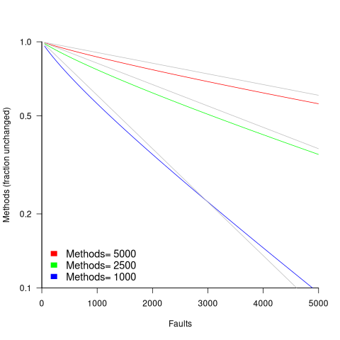
The plot below shows the predicted fraction of unmodified methods against number of faults, for programs of various sizes; the grey lines show the rough approximation:  (code+data):
The observed behavior of most reported faults involving a subset of a program’s methods can be modelled using some form of preferential attachment.
One preferential attachment model specifies that the likelihood of a coding mistake appearing in a method is proportional to ") , where
, where  is the number of previously detected coding mistakes in the method.
The estimated number of unmodified methods is now:
}Li_b(({M zeta(b-1)}/{M zeta(b-1)+a*(F+1) zeta(b)})^{1/a})")
where:  is the average value of
  over all faults (if
  , then
  for a power law with exponent 2.35).
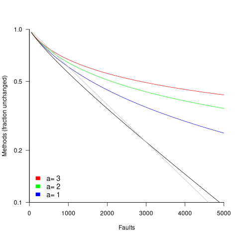
The plot below shows the predicted fraction of unmodified methods against number of faults for a program containing 1,000 methods, for various values of , with the black line showing the fraction of unmodified methods predicted by the simple model above (code+data):
In practice, random selection of the method containing a coding mistake will introduce some fuzziness in the predicted fraction of unmodified methods.
As the number of reported faults grows, the attraction of methods involved in previous reported faults slows the rate at which methods experience their first detected coding mistake.
How realistic are these models?
By focusing on the number of unmodified methods, many complications are avoided.
Both models assume that an unchanging number of methods in a program and that the length of each method is fixed. This assumption holds between each release of a program.
For actively maintained programs, the number of methods in a program changes over time, and the length of some existing methods also changes (if a program were not actively maintained, reported faults would not get fixed).
These models are unlikely to be applicable to programs with short release cycles, where there are few reported faults between releases.
How well do the models’ predictions agree with the data?
At the moment, I am not aware of a dataset containing the appropriate data. Number of faults vs unmodified methods has been added to my list of interesting patterns to notice.
Summary of the derivation of the solutions for the two models.
Simple model
The expected number of unmodified methods, ") , is:
, is:
=sum{L=1}{T}{m_L{P(U_LF)}}") , where
, where  is the length of the longest method,
  is the number of methods of length , and
 ") is the probability that a method of length will be unmodified after fault reports.
is the probability that a method of length will be unmodified after fault reports.
The evidence shows that the distribution of methods containing a given number of lines, , is well-fitted by a power law (for Java: ).
Given a program containing methods, the number of methods of length is:
 , where for Java.
If is large and  , then the sum can be approximated by the Riemann zeta function, , giving:
}}")
The probability that a method containing lines will not be modified by a fault report (assuming that fixing the mistake only involves one method) is:  , where
  is the total lines of code in the program, and the probability of this method not being modified after fault reports is approximately:
^F approx e^{{-F*L}/{P_t}}")
The expected number of empty boxes is:
}}*e^{{-F*L}/{P_t}}}=M/{zeta(b)}Li_b(e^{-F/{P_t}})")
The number of lines of code in a program containing methods is:
}}}=M/{zeta(b)}sum{L=1}{T}{L^{1-b}}=M{{zeta(b-1)}/{zeta(b)}}")
Finally giving:
}Li_b(e^{-{F/M}{{zeta(b)}/{zeta(b-1)}}})")
where is the polylogarithm function.
This equation is roughly, for the purposes of understanding the effect of each variable:

Preferential attachment model
When a mistake is corrected in a method, the attraction weight of that method increases (alternatively, the attraction weight of the other methods decreases). The probability that a method is not modified after fault reports is now:
}=prod{k=0}{F}{{P_t+a*k-L}/{P_t+a*k}}={Gamma({P_t}/a)Gamma({P_t-L}/a+F+1)}/{Gamma({P_t-L}/a)Gamma(P_t/a+F+1)}")
where:  the average value of over all faults, and
  is the gamma function.
applying the Stirling/Gamma–ratio rule, i.e., }/{Gamma(z+b)} approx z^{a-b}") we get:
we get:
})^{F/a} = ((P_t/{P_t+a*(F+1)})^{1/a})^F")
where the expression ^{1/a})^F") is the preferential attachment version of the expression
is the preferential attachment version of the expression ^F") appearing in the simple model derivation. Using this preferential attachment expression in the analysis of the simple model, we get:
appearing in the simple model derivation. Using this preferential attachment expression in the analysis of the simple model, we get:
I don’t have a rough approximation for this expression.
Impact of developer uncertainty on estimating probabilities
For over 50 years, it has been known that people tend to overestimate the likelihood of uncommon events/items occurring, and underestimate the likelihood of common events/items. This behavior has replicated in many experiments and is sometimes listed as a so-called cognitive bias.
Cognitive bias has become the term used to describe the situation where the human response to a problem (in an experiment) fails to match the response produced by the mathematical model that researchers believe produces the best output for this kind of problem. The possibility that the mathematical models do not reflect the reality of the contexts in which people have to solve the problems (outside of psychology experiments), goes against the grain of the idealised world in which many researchers work.
When models take into account the messiness of the real world, the responses are a closer match to the patterns seen in human responses, without requiring any biases.
The 2014 paper Surprisingly Rational: Probability theory plus noise explains biases in judgment by F. Costello and P. Watts (shorter paper), showed that including noise in a probability estimation model produces behavior that follows the human behavior patterns seen in practice.
If a developer is asked to estimate the probability that a particular event,  , occurs, they may not have all the information needed to make an accurate estimate. They may fail to take into account some s, and incorrectly include other kinds of events as being s. This noise,
  , introduces a pattern into the developer estimate:
*P_E + N*(1-P_E)=(1-2N)*P_E+N")
where:  is the developer’s estimated probability of event occurring,
  is the actual probability of the event, and is the probability that noise produces an incorrect classification of an event as
  or (for simplicity, the impact of noise is assumed to be the same for both cases).
The plot below shows actual event probability against developer estimated probability for various values of , with a red line showing that at  , the developer estimate matches reality (code):

The effect of noise is to increase probability estimates for events whose actually probability is less than 0.5, and to decrease the probability when the actual is greater than 0.5. All estimates move towards 0.5.
What other estimation behaviors does this noise model predict?
If there are two events, say  and
and  , then the noise model (and probability theory) specifies that the following relationship holds:
+P(B) == P(A & B)+P(A delim{|}{B}{})")
where: ") denotes the probability of its argument.
denotes the probability of its argument.
The experimental results show that this relationship does hold, i.e., the noise model is consistent with the experiment results.
This noise model can be used to explain the conjunction fallacy, i.e., Tversky & Kahneman’s famous 1970s “Lindy is a bank teller” experiment.
What predictions does the noise model make about the estimated probability of experiencing  (
( ) occurrences of the event in a sequence of
  assorted events (the previous analysis deals with the case
  )?
)?
An estimation model that takes account of noise gives the equation:

where:  is the developer’s estimated probability of experiencing s in a sequence of length , and
  is the actual probability of there being .
The plot below shows actual event probability against developer estimated probability for various values of , with a red line showing that at , the developer estimate matches reality (code):

This predicted behavior, which is the opposite of the case where , follows the same pattern seen in experiments, i.e., actual probabilities less than 0.5 are decreased (towards zero), while actual probabilities greater than 0.5 are increased (towards one).
There have been replications and further analysis of the predictions made by this model, along with alternative models that incorporate noise.
To summarise:
When estimating the probability of a single event/item occurring, noise/uncertainty will cause the estimated probability to be closer to 50/50 than the actual probability.
When estimating the probability of multiple events/items occurring, noise/uncertainty will cause the estimated probability to move towards the extremes, i.e., zero and one.
Calculating statement execution likelihood
In the following code, how often will the variable b be incremented, compared to a?
If we assume that the variables x and y have values drawn from the same distribution, then the condition (x < y) will be true 50% of the time (ignoring the situation where both values are equal), i.e., b will be incremented half as often as a.
a++; if (x < y) { b++; if (x < z) { c++; } } |
If the value of z is drawn from the same distribution as x and y, how often will c be incremented compared to a?
The test (x < y) reduces the possible values that x can take, which means that in the comparison (x < z), the value of x is no longer drawn from the same distribution as z.
Since we are assuming that z and y are drawn from the same distribution, there is a 50% chance that (z < y).
If we assume that (z < y), then the values of x and z are drawn from the same distribution, and in this case there is a 50% change that (x < z) is true.
Combining these two cases, we deduce that, given the statement a++; is executed, there is a 25% probability that the statement c++; is executed.
If the condition (x < z) is replaced by (x > z), the expected probability remains unchanged.
If the values of x, y, and z are not drawn from the same distribution, things get complicated.
Let's assume that the probability of particular values of x and y occurring are  and
and  , respectively. The constants
  and
and  are needed to ensure that both probabilities sum to one; the exponents
  and
and  control the distribution of values. What is the probability that
 (x < y) is true?
Probability theory tells us that  = int{-infty}{+infty} f_B(x) F_A(x) dx") , where:
, where:  is the probability distribution function for (in this case:
  ), and
  the cumulative probability distribution for (in this case:
 ") ).
).
Doing the maths gives the probability of (x < y) being true as:  .
.
The (x < z) case can be similarly derived, and combining everything is just a matter of getting the algebra right; it is left as an exercise to the reader :-)
Quality of data analysis: two recent papers
Software engineering research has and continues to suffer from very low quality data analysis. The underlying problem is that practitioners are happy to go along with the status quo, not bothering to learn basic statistics or criticize data analysis in papers they are asked to review. Two recent papers I have read spring out as being at opposite ends of the spectrum.
In their paper A replicated survey of IT software project failures Khaled El Emam and A. Günes Koru don’t just list the mean values for the responses they get they also give the 95% confidence bounds on those values. At a superficial level this has the effect of making their results look much less interesting; for instance a quick glance at Table 3 “Reasons for project cancellation” suggests there is a significant difference between “Lack of necessary technical skills” at 22% and “Over schedule” at 17% but a look at the 95% confidence bounds, (6%–48%) and (4%–41%) respectively, shows that almost nothing can be said about the relative contribution of these two reasons (why publish these numbers, because nothing else has been published and somebody has to start somewhere). The authors understand the consequences of using a small sample size and have the integrity to list the confidence bounds rather than leave the reader to draw completely unjustified conclusions. I wish everybody was as careful and upfront about their analysis as these authors.
The paper Assessing Programming Language Impact on Development and Maintenance: A Study on C and C++ by Pamela Bhattacharya and Iulian Neamtiu takes some interesting ideas and measurements and completely mangles the statistical analysis (something the conference’s reviewers should have picked up on).
I encourage everybody to measure code and do statistical analysis. It looks like what happened here is that a PhD student got in over her head and made lots of mistakes, something that happens to us all when learning a new subject. The problem is that these mistakes made it through into a published paper and its conclusions are likely to repeated (these conclusions may or may not be true and it may or may not be possible to reliably test them from the data gathered, but the analysis presented in the paper faulty and so its conclusions cannot be trusted). I hope the authors will reanalyze their data using the appropriate techniques and publish an updated version of the paper.
Some of the hypothesis being tested include:
- C++ is replacing C as a main development language. The actual hypothesis tested is the more interesting question: “Is the percentage of C++ in projects that also contain substantial amounts of C growing at the expense of C?”
So the unit of measurement is the project and only four of these are included in the study; an extremely small sample size that must have an error bound of around 50% (no mention of error bounds in the paper). The analysis of the data claims to use linear regression but seems completely confused, lets not get bogged down in the details but move on to other more obvious mistakes.
- C++ code is of higher internal quality than C code. The data consists of various source code metrics, ignoring whether these are a meaningful measure of quality, lets look at how the numbers are analysed. I was somewhat surprised to read: “the distributions of complexity values … are skewed, thus arithmetic mean is not the right indicator of an ongoing trend. Therefore, …, we use the geometric mean …” While the arithmetic mean might not be a useful indicator (I have trouble seeing why not), use of the geometric mean is bizarre and completely wrong. Because of its multiplicative nature the geometric mean of a set of values having a fixed arithmetic mean decreases as its variance increases. For instance, the two sets of values (40, 60) and (20, 80) both have an arithmetic mean of 50, while their geometric means are 48.98979 (i.e.,
^0.5") ) and 40 (i.e.,
) and 40 (i.e., ^0.5") ) respectively.
) respectively.
So if anything can be said about the bizarre idea of comparing the geometric mean of complexity metrics as they change over time, it is that increases/decreases are an indicator of decrease/increase in variance of the measurements.
- C++ code is less prone to bugs than C code. The statistical analysis here made a common novice mistake. The null hypothesis tested was: “C code has lower or equal defect density than C++ code.” and this was rejected. The incorrect conclusion drawn was that “C++ code is less prone to bugs than C code.” Statistically one does not follow from the other, the data could be inconclusive and the researchers should have tested this question as the null hypothesis if this is the claim they wanted to make. There are also lots of question marks over other parts of the analysis, but this is the biggest blunder.
Christmas books for 2009
I thought it would be useful to list the books that gripped me one way or another this year (and may be last year since I don’t usually track such things closely); perhaps they will give you some ideas to add to your Christmas present wish list (please make your own suggestions in the Comments). Most of the books were published a few years ago, I maintain piles of books ordered by when I plan to read them and books migrate between piles until eventually read. Looking at the list I don’t seem to have read many good books this year, perhaps I am spending too much time reading blogs.
These books contain plenty of facts backed up by numbers and an analytic approach and are ordered by physical size.
The New Science of Strong Materials by J. E. Gordon. Ideal for train journeys since it is a small book that can be read in small chunks and is not too taxing. Offers lots of insight into those properties of various materials that are needed to build things (‘new’ here means postwar).
Europe at War 1939-1945 by Norman Davies. A fascinating analysis of the war from a numbers perspective. It is hard to escape the conclusion that in the grand scheme of things us plucky Brits made a rather small contribution, although subsequent Hollywood output has suggested otherwise. Also a contender for a train book.
Japanese English language and culture contact by James Stanlaw. If you are into Japanese culture you will love this, otherwise avoid.
Evolutionary Dynamics by Martin A. Nowak. For the more mathematical folk and plenty of thought power needed. Some very powerful general results from simple processes.
Analytic Combinatorics by Philippe Flajolet and Robert Sedgewick. Probably the toughest mathematical book I have kept at (yet to get close to the end) in a few years. If number sequences fascinate you then give it a try (a pdf is available).
Probability and Computing by Michael Mitzenmacher and Eli Upfal. For the more mathematical folk and plenty of thought power needed. Don’t let the density of Theorems put you off, the approach is broad brush. Plenty of interesting results with applications to solving problems using algorithms containing a randomizing component.
Network Algorithmics by George Varghese. A real hackers book. Not so much a book about algorithms used to solve networking problems but a book about making engineering trade-offs and using every ounce of computing functionality to solve problems having severe resource and real-time constraints.
Virtual Machines by James E. Smith and Ravi Nair. Everything you every wanted to know about virtual machines and more.
Biological Psychology by James W. Kalat. This might be a coffee table book for scientists. Great illustrations, concise explanations, the nuts and bolts of how our bodies runs at the protein/DNA level.
Estimating variance when measuring source
Yesterday I finally delivered a paper on if/switch usage measurements to the ACCU magazine editor and today I read about a switch statement usage that, if common, would invalidate a chunk of my results. Does anything jump out at you in the following snippet?
switch (x) { case 1: { z++; ... break; } ... |
Yes, those { } delimiting the case-labeled statement sequence. A quick check of my C source benchmarks showed this usage occurring in around 1% of case-labels. Panic over.
What is the statistical significance, i.e., variance, of that 1%? Have I simply measured an unrepresentative sample, what would be a representative sample and what would be the expected variance within a representative sample?
I am interested in commercial software development, and so I have selected half a dozen or so largish code bases as my source benchmark, preferably written in a commercial environment even if currently available as Open source. I would prefer this benchmark to be an order of magnitude larger, and perhaps I will get around to adding more programs soon.
My if/switch measurements were aimed at finding usage characteristics that varied between the two kinds of selection statements. One characteristic measured was the number of equality tests in the associated controlling expression. For instance, in:
if (x == 1 || x == 2) z--; else if (x == 3) z++; |
the first controlling expression contains two equality tests, and the second one equality test.
Plotting the percentage of equality tests that occur in the controlling expressions of if-if/if-else-if sequences and switch statements, we get the following:
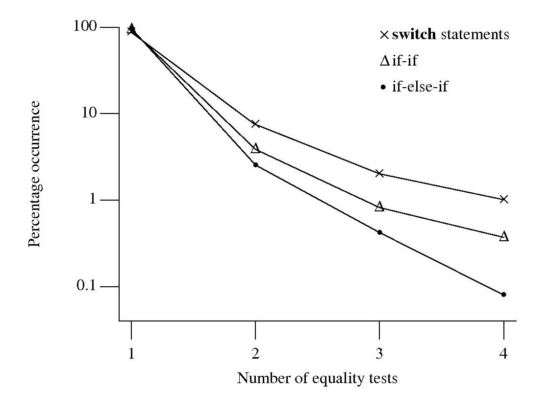
Do these results indicate that if-if/if-else-if sequences and switch statements differ in the number of equality tests contained in their controlling expressions? If I measured a completely different set of source code, would the results be very different?
To answer this question, a probability model is needed. Take as an example, the controlling expressions present in an if-if sequence. If each controlling expression is independent of the others, then the probability of two equality tests, for instance, occurring in any of these expressions is constant and thus given a large sample the distribution of two equality tests in the source has a binomial distribution. The same argument can be applied to other numbers of equality tests and other kinds of sequence.

For each measurement point in the above plot the associated error bars span the square-root of the variance of that point (assuming a binomial distribution, for a normal distribution the length of this span is known as the standard deviation). The error bars overlap, suggesting that the apparent difference in percentage of equality tests in each kind of sequence is not statistically significant.
The existence of some dependency between controlling expression equality tests would invalidate this simply analysis, or at least reduce its reliability. I did notice that in a sequence that containing two equality tests, the controlling expression that contained it tended to appear later in the sequence (the reverse of the example given above). Did I notice this because I tend to write this way? A question for another day.
What I changed my mind about in 2008
A few years ago The Edge asked people to write about what important issue(s) they had recently changed their mind about. This is an interesting question and something people ought to ask themselves every now and again. So what did I change my mind about in 2008?
1. Formal verification of nontrivial C programs is a very long way off. A whole host of interesting projects (e.g., Caduceus, Comcert and Frame-C) going on in France has finally convinced me that things are a lot closer than I once thought. This does not mean that I think developers/managers will be willing to use them, only that they exist.
2. Automatically extracting useful information from source code identifier names is still a long way off. Yes, I am a great believer in the significance of information contained in identifier names. Perhaps because I have studied the issues in detail I know too much about the problems and have been put off attacking them. A number of researchers (e.g., Emily Hill, David Shepherd, Adrian Marcus, Lin Tan and a previously blogged about project) have simply gone ahead and managed to extract (with varying amount of human intervention) surprising amounts of useful from identifier names.
3. Theoretical analysis of non-trivial floating-point oriented programs is still a long way off. Daumas and Lester used the Doobs-Kolmogorov Inequality (I had to look it up) to deduce the probability that the rounding error in some number of floating-point operations, within a program, will exceed some bound. They also integrated the ideas into NASA’s PVS system.
You can probably spot the pattern here, I thought something would not happen for years and somebody went off and did it (or at least made an impressive first step along the road). Perhaps 2008 was not a good year for really major changes of mind, or perhaps an earlier in the year change of mind has so ingrained itself in my mind that I can no longer recall thinking otherwise.
Distribution of numeric values (additive)
Developers and testers rarely put any thought into working out the likely distribution of numeric values (final or intermediate) computed during the execution of the code they write.
The likely value of a variable is useful to know in a number of situations, including optimizing code (should it prove to be necessary) for the common case and testing (what distribution of input values are needed to be confident that all paths through a program are exercised?)
The answer for the ‘simple’ distributions is actually more complicated to work with than the more ‘complicated’ distributions. For instance, the sum of two independent values having a normal distributions is a normal distribution and the sum of two Poisson distributions is also a Poisson distribution.
What if the values are uniformly distributed? If two independent, randomly chosen, uniformly distributed, variables, are added what is the distribution of the result? For instance, if the values of X and Y are independent of each other and take on any value between 0 and 9, with equal likelihood, what is the most (and least) likely value of X+Y?
Warning: Information spoilers follow.
You are probably thinking that the result will also be uniformly distributed and indeed it would be if the range of values taken by X and Y did not overlap. When the possible range of values overlap exactly the answer is the triangular distribution, with the mostly likely result being 9 and the least likely results being 0 and 18.
The variance of the actual result distribution is approximately six times smaller than the original distribution, meaning that the common cases occupy a much narrower value range. This value range ‘narrowing’ goes someway towards helping to explain the surprising discovery that during program execution a small set of (integer and floating) values often occur with such regularity that it might be worth cpu arithmetic units remembering previous operands and their results (i.e., to save time by returning the result rather than recalculating it).
Recent Comments