Archive
Modelling time to next reported fault
After the arrival of a fault report for a program, what is the expected elapsed time until the next fault report arrives (assuming that the report relates to a coding mistake and is not a request for enhancement or something the user did wrong, and the number of active users remains the same and the program is not changed)? Here, elapsed time is a proxy for amount of program usage.
Measurements (here and here) show a consistent pattern in the elapsed time of duplicate reports of individual faults. Plotting the time elapsed between the first report and the n’th report of the same fault in the order they were reported produces an exponential line (there are often changes in the slope of this line). For example, the plot below shows 10 unique faults (different colors), the number of days between the first report and all subsequent reports of the same fault (plus character); note the log scale y-axis (discussed in this post; code+data):

The first person to report a fault may experience the same fault many times. However, they only get to submit one report. Also, some people may experience the fault and not submit a report.
If the first reporter had not submitted a report, then the time of first report would be later. Also, the time of first report could have been earlier, had somebody experienced it earlier and chosen to submit a report.
The subpopulation of users who both experience a fault and report it, decreases over time. An influx of new users is likely to cause a jump in the rate of submission of reports for previously reported faults.
It is possible to use the information on known reported faults to build a probability model for the elapsed time between the last reported known fault and the next reported known fault (time to next reported unknown fault is covered at the end of this post).
The arrival of reports for each distinct fault can be modelled as a Poisson process. The time between events in a Poisson process with rate  has an exponential distribution, with mean
  . The distribution of a sum of multiple Poisson processes is itself a Poisson process whose rate is the sum of the individual rates. The other key point is that this process is memoryless. That is, the elapsed time of any report has no impact on the elapsed time of any other report.
If there are  different faults whose fitted report time exponents are:
  ,
,  …
…  , then summing the Poisson rates,
  , gives the mean
  , for a probability model of the estimated time to next any-known fault report.
To summarise. Given enough duplicate reports for each fault, it’s possible to build a probability model for the time to next known fault.
In practice, people are often most interested in the time to the first report of a previous unreported fault.
tl;dr Modelling time to next previously unreported fault has an analytic solution that depends on variables whose values have to be approximately approximated.
The method used to build a probability model of reports of known fault can be used extended to build a probability model of first reports of currently unknown faults. To build this model, good enough values for the following quantities are needed:
- the number of unknown faults,
 , remaining in the program. I have some ideas about estimating the number of unknown faults, , and will discuss them in another post,
 - the time,
 , needed to have received at least one report for each of the unknown faults. In practice, this is the lifetime of the program, and there is data on software half-life. However, all coding mistakes could trigger a fault report, but not all coding mistakes will have done so during a program’s lifetime. This is a complication that needs some thought,
 - the values of
 ,
,  …
…  for each of the unknown faults. There is some data suggesting that these values are drawn from an exponential distribution, or something close to one. Also, an equation can be fitted to the values of the known faults. The analysis below assumes that the
  for each unknown fault that might be reported is randomly drawn from an exponential distribution whose mean is .
This rate will be affected by program usage (i.e., number of users and the activities they perform), and source code characteristics such as the number of executions paths that are dependent on rarely true conditions.
Putting it all together, the following is the question I asked various LLMs (which uses  , rather than ):
There are independent processes. Each process,  , transmits a signal, and the number of signals transmitted in a fixed time interval, , has a Poisson distribution with mean
  for
for  . The values are randomly drawn from the same exponential distribution. What is the cumulative distribution for the time between the successive first signals from the processes.
The cumulative distribution gives the probability that an event has occurred within a given amount of time, in this case the time since the last fault report.
The ChatGPT 5.2 Thinking response (Grok Thinking gives the same formula, but no chain of thought): The probability that the  unknown fault is reported within time
  of the previous report of an unknown fault,
 ") , is given by the following rather involved formula:
, is given by the following rather involved formula:
=1-(a/{a+t})^{N-k}{}_{2}F_1(N-k, k; N+1; t/{a+t})")
where: is the initial number of faults that have not been reported,  , and
, and  is the hypergeometric function.
The important points to note are: the value  decreases as more unknown faults are reported, and the dominant contribution of the value .
Deepseek’s response also makes complicated use of the same variables, and the analysis is very similar before making some simplifications that don’t look right (text of response). Kimi’s response is usually very good, but for this question failed to handle the consequences of .
Almost all published papers on fault prediction ignore the impact of number of users on reported faults, and that report time for each distinct fault has a distinct distribution, i.e., their analysis is not connected to reality.
Percentage of methods containing no reported faults
It is often said, with some evidence, that 80% of reported faults, for a program, occur in 20% of its code. I think this pattern is a consequence of 20% of the code being executed 80% of the time, while many researchers believe that 20% of the source code has characteristics that result in it containing 80% of the coding mistakes.
The 20% figure is commonly measured as a percentage of methods/functions, rather than a percentage of lines of code.
This post investigates the expected fraction of a program’s methods that remain fault report free, based on two probability models.
Both models assume that coding mistakes are uniformly scattered throughout the code (i.e., every statement has the same probability of containing a mistake) and that the corresponding coding mistake is contained within a single method (the evidence suggests that this is true for 50% of faults).
A simple model is to assume that when a new fault is reported, the probability that the corresponding coding mistake appears in a particular method is proportional to the method’s length,  in lines of code, of the method. The evidence shows that the distribution of methods containing a given number of lines, , is well-fitted by a power law (for Java:
  ).
).
If  reported faults have been fixed in a program containing
  methods/functions, what is the expected number of methods that have not been modified by the fixing process?
The answer (with help from: mostly Kimi, with occasional help from Deepseek (who don’t have a share chat options), ChatGPT 5, Grok, and some approximations; chat logs) is:
}Li_b(e^{-{F/M}{{zeta(b)}/{zeta(b-1)}}})")
where:  is the Riemann zeta function,
  is the polylogarithm function and
  for Java.
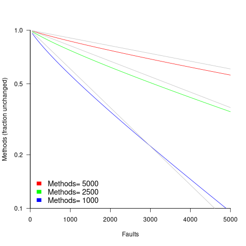
The plot below shows the predicted fraction of unmodified methods against number of faults, for programs of various sizes; the grey lines show the rough approximation:  (code+data):
The observed behavior of most reported faults involving a subset of a program’s methods can be modelled using some form of preferential attachment.
One preferential attachment model specifies that the likelihood of a coding mistake appearing in a method is proportional to ") , where
, where  is the number of previously detected coding mistakes in the method.
The estimated number of unmodified methods is now:
}Li_b(({M zeta(b-1)}/{M zeta(b-1)+a*(F+1) zeta(b)})^{1/a})")
where:  is the average value of
  over all faults (if
  , then
  for a power law with exponent 2.35).
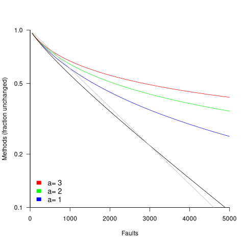
The plot below shows the predicted fraction of unmodified methods against number of faults for a program containing 1,000 methods, for various values of , with the black line showing the fraction of unmodified methods predicted by the simple model above (code+data):
In practice, random selection of the method containing a coding mistake will introduce some fuzziness in the predicted fraction of unmodified methods.
As the number of reported faults grows, the attraction of methods involved in previous reported faults slows the rate at which methods experience their first detected coding mistake.
How realistic are these models?
By focusing on the number of unmodified methods, many complications are avoided.
Both models assume that an unchanging number of methods in a program and that the length of each method is fixed. This assumption holds between each release of a program.
For actively maintained programs, the number of methods in a program changes over time, and the length of some existing methods also changes (if a program were not actively maintained, reported faults would not get fixed).
These models are unlikely to be applicable to programs with short release cycles, where there are few reported faults between releases.
How well do the models’ predictions agree with the data?
At the moment, I am not aware of a dataset containing the appropriate data. Number of faults vs unmodified methods has been added to my list of interesting patterns to notice.
Summary of the derivation of the solutions for the two models.
Simple model
The expected number of unmodified methods, ") , is:
, is:
=sum{L=1}{T}{m_L{P(U_LF)}}") , where is the length of the longest method,
, where is the length of the longest method,  is the number of methods of length , and
 ") is the probability that a method of length will be unmodified after fault reports.
is the probability that a method of length will be unmodified after fault reports.
The evidence shows that the distribution of methods containing a given number of lines, , is well-fitted by a power law (for Java: ).
Given a program containing methods, the number of methods of length is:
 , where for Java.
If is large and  , then the sum can be approximated by the Riemann zeta function, , giving:
}}")
The probability that a method containing lines will not be modified by a fault report (assuming that fixing the mistake only involves one method) is:  , where
  is the total lines of code in the program, and the probability of this method not being modified after fault reports is approximately:
^F approx e^{{-F*L}/{P_t}}")
The expected number of empty boxes is:
}}*e^{{-F*L}/{P_t}}}=M/{zeta(b)}Li_b(e^{-F/{P_t}})")
The number of lines of code in a program containing methods is:
}}}=M/{zeta(b)}sum{L=1}{T}{L^{1-b}}=M{{zeta(b-1)}/{zeta(b)}}")
Finally giving:
}Li_b(e^{-{F/M}{{zeta(b)}/{zeta(b-1)}}})")
where is the polylogarithm function.
This equation is roughly, for the purposes of understanding the effect of each variable:

Preferential attachment model
When a mistake is corrected in a method, the attraction weight of that method increases (alternatively, the attraction weight of the other methods decreases). The probability that a method is not modified after fault reports is now:
}=prod{k=0}{F}{{P_t+a*k-L}/{P_t+a*k}}={Gamma({P_t}/a)Gamma({P_t-L}/a+F+1)}/{Gamma({P_t-L}/a)Gamma(P_t/a+F+1)}")
where:  the average value of over all faults, and
  is the gamma function.
applying the Stirling/Gamma–ratio rule, i.e., }/{Gamma(z+b)} approx z^{a-b}") we get:
we get:
})^{F/a} = ((P_t/{P_t+a*(F+1)})^{1/a})^F")
where the expression ^{1/a})^F") is the preferential attachment version of the expression
is the preferential attachment version of the expression ^F") appearing in the simple model derivation. Using this preferential attachment expression in the analysis of the simple model, we get:
appearing in the simple model derivation. Using this preferential attachment expression in the analysis of the simple model, we get:
I don’t have a rough approximation for this expression.
Predicting the future with data+logistic regression
Predicting the peak of data fitted by a logistic equation is attracting a lot of attention at the moment. Let’s see how well we can predict the final size of a software system, in lines of code, using logistic regression (code+data).
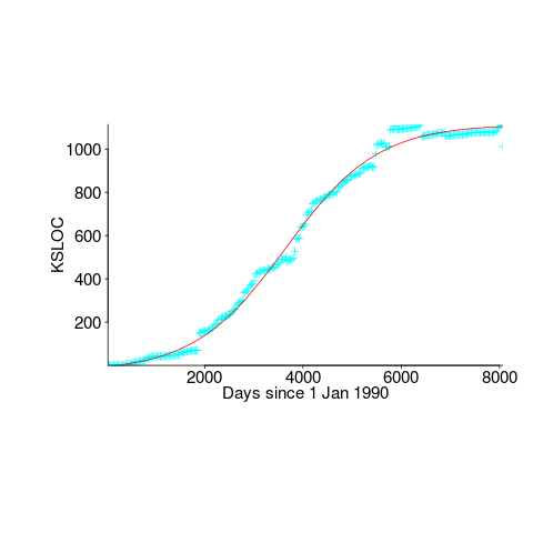
First up is the size of the GNU C library. This is not really a good test, since the peak (or rather a peak) has been reached.
We need a system that has not yet reached an easily recognizable peak. The Linux kernel has been under development for many years, and lots of LOC counts are available. The plot below shows a logistic equation fitted to the kernel data, assuming that the only available data was up to day: 2,900, 3,650, 4,200, and 5,000+ (code+data). Can you tell which fitted line corresponds to which number of days?
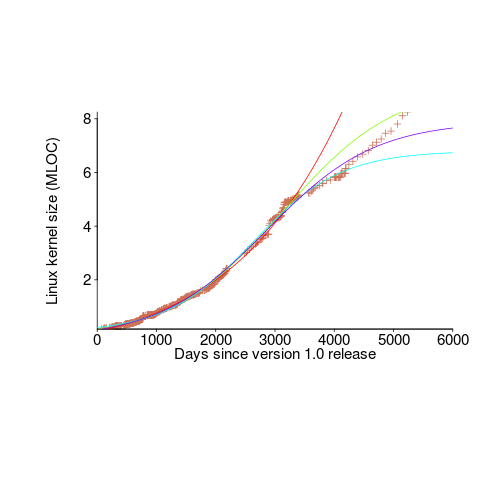
The underlying ‘problem’ is that we are telling the fitting software to fit a particular equation; the software does what it has been told to do, and fits a logistic equation (in this case).
A cubic polynomial is also a great fit to the existing kernel data (red line to the left of the blue line), and this fitted equation can be extended into future (to the right of the blue line); dotted lines are 95% confidence bounds. Do any readers believe the future size of the Linux kernel predicted by this cubic model?
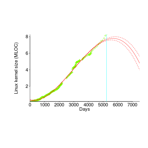
Predicting the future requires lots of data on the underlying processes that drive events. Modelling events is an iterative process. Build a model, check against reality, adjust model, rinse and repeat.
If the COVID-19 experience trains people to be suspicious of future predictions made by models, it will have done something positive.
Time taken to compile a source file
How long will it take to compile a source file?
When computers were a lot slower than they are today, this question was of general interest. Job scheduling is more effective when reliable runtime estimates are available, and developers want to know if there is enough time to get a coffee before the compile finishes.
An embarrassing fact about compile time performance, used to be that a large percentage of compile time was spent doing lexical analysis [“The cost of lexical analysis”, I cannot find an online copy]. Why was this embarrassing? Compiler writers like to boast about all the fancy optimizations their compiler does; but doing fancy stuff consumes lots of resources, so why were compilers spending so much of their time doing simple things like lexical analysis? The reality was that fancy compiler optimizations were not commercially viable until developer computers contained tens of megabytes of memory, i.e., very few pre-1990 compilers did any real optimization (people are still fussing over lexer performance).
An analysis of the data in Captain Dennis Miller’s Masters thesis (late Rome period), finds compile time is proportional to the square root of the number of tokens in the source (code+data); more complicated models are a slightly better fit. Where did square root come from? I expected a linear relationship, but would be willing to go with log. The measurements are from Ada compilers in the mid 1980s. I know several people who worked on Ada compilers during that time, and they were implementing the latest fancy optimizations (Ada was going to be the next big thing and the venture capital was flowing; big companies, with big computers were going to be paying lots of money to use Ada, but then microcomputers came along). I think that square root is driven by OS resource limitations, the compilers are using lots of memory and a noticeable amount of time is spent swapping.
So computers got a lot faster and people lost interest in estimates of how long it would take to compile individual files. I have not seen any interest in predicting how long it would take to compile whole projects (just complaints about how long it takes). There has been some work on progress indicators, updated as compilation progresses, which is a step in the right direction. Perhaps somebody has recorded compile time information and thrown machine learning at it; I usually ignore machine learning papers applied to software engineering and perhaps I have missed something. Pointers to project compile time prediction work welcome.
Then along came just-in-time compilation. Now people want to estimate how long it will take to generate machine code from some intermediate form, that is being interpreted.
The plot below (thanks to Rafael Auler for kindly supplying the data from his paper) shows the time taken to generate code from functions containing a given number of LLVM instructions (an intermediate code), at optimization level O3. The red line is a regression fit to one of the ‘arms’ and shows constant time for less than 100’ish instructions and then a linear relationship. I have no idea why the time is roughly constant for a large number of functions.
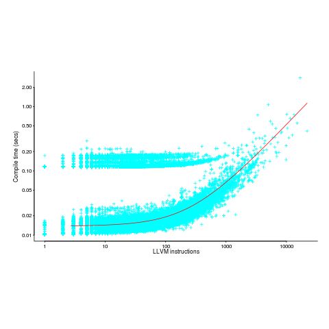
There is a lot of variation for function containing the same number of instructions. This is to be expected when lots of different optimizations are being tried; sometimes a function will contain lots of the kind of code that a particular optimization spends lot of times process and sometimes the code will not contain anything interesting (i.e., no optimizations are found).
Predictive Modeling: 15th COW workshop
I was at a very interesting workshop on Predictive Modelling and Search Based Software Engineering on Monday/Tuesday this week, and I am going to say something about the talks that interested me. The talks were recorded, and the videos will appear on the website in a few weeks. The CREST Open Workshop (COW) runs roughly once a month and the group leader, Mark Harman, is always on the lookout for speakers, do let him know if you are in the area.
- Tim Menzies talked about how models built from one data set did well on that dataset but often not nearly as well on another (i.e., local vs global applicability of models). Academics papers usually fail to point out that any results might not be applicable outside the limited domain examined, in fact they often give the impression of being generally applicable.
Me: Industry likes global solutions because it makes life simpler and because local data is often not available. It is a serious problem if, for existing methods, data on one part of a companies’ software development activity is of limited use in predicting something about a different development activity in the same company and completely useless at predicting things at a different company.
- Yuriy Brun talked about something that is so obviously a good idea, it is hard to believe that it had not been done years ago. The idea is to have your development environment be aware of what changes other software developers have made to their local copies of source files you also have checked out from version control. You are warned as soon your local copy conflicts with somebody else’s local copy, i.e., a conflict would occur if you both check in your local copy to the central repository. This warning has the potential to save lots of time by having developers talk to each about resolving the conflict before doing any more work that depends on the conflicting change.
Crystal is a plug-in for Eclipse that implements this functionality, and Visual Studio support is expected in a couple of releases time.
I have previously written about how multi-core processors will change software development tools, and I think this idea falls into that category.
- Martin Shepperd presented a very worrying finding. An analysis of the results published in 18 papers dealing with fault prediction found that the best predictor (over 60%) of agreement between results in different papers was co-authorship. That is, when somebody co-authored a paper with another person, any other papers they published were more likely to agree with other results published by that person than with results published by somebody they had not co-authored a paper with. This suggests that each separate group of authors is doing something different that significantly affects their results; this might be differences in software packages being used, differences in configuration options or tuning parameters, so something else.
It might be expected that agreement between results would depend on the techniques used, but Shepperd et al’s analysis found this kind of dependency to be very small.
An effect is occurring that is not documented in the published papers; this is not how things are supposed to be. There was lots of interest in obtaining the raw data to replicate the analysis.
- Camilo Fitzgerald talked about predicting various kinds of feature request ‘failures’ and presented initial results based on data mined from various open source projects; possible ‘failures’ included a new feature being added and later removed and significant delay (e.g., 1 year) in implementing a requested feature. I have previously written about empirical software engineering only being a few years old and this research is a great example of how whole new areas of research are being opened up by the availability of huge amounts of data on open source projects.
One hint for PhD students: It is no good doing very interesting work if you don’t keep your web page up to date, so people can find out more about it
I talked to people who found other presentations very interesting. They might have failed to catch my eye because my interest or knowledge of the subject is low or I did not understand their presentation (a few gave no background or rationale and almost instantly lost me); sometimes the talks during coffee were much more informative.
Recent Comments