Archive
Moore’s law was a socially constructed project
Moore’s law was a socially constructed project that depended on the coordinated actions of many independent companies and groups of individuals to last for as long it did.
All products evolve, but what was it about Moore’s law that enabled microelectronics to evolve so much faster and for longer than most other products?
Moore’s observation, made in 1965 based on four data points, was that the number of components contained in a fabricated silicon device doubles every year. The paper didn’t make this claim in words, but a line fitted to four yearly data points (starting in 1962) suggested this behavior continuing into the mid-1970s. The introduction of IBM’s Personal Computer, in 1981 containing Intel’s 8088 processor, led to interested parties coming together to create a hugely profitable ecosystem that depended on the continuance of Moore’s law.
The plot below shows Moore’s four points (red) and fitted regression model (green line). In practice, since 1970, fitting a regression model (purple line) to the number of transistors in various microprocessors (blue/green, data from Wikipedia), finds that the number of transistors doubled every two years (code+data):

In the early days, designing a device was mostly a manual operation; that is, the circuit design and logic design down to the transistor level were hand-drawn. This meant that creating a device containing twice as many transistors required twice as many engineers. At some point the doubling process either becomes uneconomic or it takes forever to get anything done because of the coordination effort.
The problem of needing an exponentially-growing number of engineers was solved by creating electronic design automation tools (EDA), starting in the 1980s, with successive generations of tools handling ever higher levels of abstraction, and human designers focusing on the upper levels.
The use of EDA provides a benefit to manufacturers (who can design differentiated products) and to customers (e.g., products containing more functionality).
If EDA had not solved the problem of exponential growth in engineers, Moore’s law would have maxed-out in the early 1980s, with around 150K transistors per device. However, this would not have stopped the ongoing shrinking of transistors; two economic factors independently incentivize the creation of ever smaller transistors.
When wafer fabrication technology improvements make it possible to double the number of transistors on a silicon wafer, then around twice as many devices can be produced (assuming unchanged number of transistors per device, and other technical details). The wafer fabrication cost is greater (second row in table below), but a lot less than twice as much, so the manufacturing cost per device is much lower (third row in table).
The doubling of transistors primarily provides a manufacturer benefit.
The following table gives estimates for various chip foundry economic factors, in dollars (taken from the report: AI Chips: What They Are and Why They Matter). Node, expressed in nanometers, used to directly correspond to the length of a particular feature created during the fabrication process; these days it does not correspond to the size of any specific feature and is essentially just a name applied to a particular generation of chips.
Node (nm) 90 65 40 28 20 16/12 10 7 5 Foundry sale price per wafer 1,650 1,937 2,274 2,891 3,677 3,984 5,992 9,346 16,988 Foundry sale price per chip 2,433 1,428 713 453 399 331 274 233 238 Mass production year 2004 2006 2009 2011 2014 2015 2017 2018 2020 Quarter Q4 Q4 Q1 Q4 Q3 Q3 Q2 Q3 Q1 Capital investment per wafer 4,649 5,456 6,404 8,144 10,356 11,220 13,169 14,267 16,746 processed per year Capital consumed per wafer 411 483 567 721 917 993 1,494 2,330 4,235 processed in 2020 Other costs and markup 1,293 1,454 1,707 2,171 2,760 2,990 4,498 7,016 12,753 per wafer |
The second economic factor incentivizing the creation of smaller transistors is Dennard scaling, a rarely heard technical term named after the first author of a 1974 paper showing that transistor power consumption scaled with area (for very small transistors). Halving the area occupied by a transistor, halves the power consumed, at the same frequency.
The maximum clock-frequency of a microprocessor is limited by the amount of heat it can dissipate; the heat produced is proportional to the power consumed, which is approximately proportional to the clock-frequency. Instead of a device having smaller transistors consume less power, they could consume the same power at double the frequency.
Dennard scaling primarily provides a customer benefit.
Figuring out how to further shrink the size of transistors requires an investment in research, followed by designing/(building or purchasing) new equipment. Why would a company, who had invested in researching and building their current manufacturing capability, be willing to invest in making it obsolete?
The fear of losing market share is a commercial imperative experienced by all leading companies. In the microprocessor market, the first company to halve the size of a transistor would be able to produce twice as many microprocessors (at a lower cost) running twice as fast as the existing products. They could (and did) charge more for the latest, faster product, even though it cost them less than the previous version to manufacture.
Building cheaper, faster products is a means to an end; that end is receiving a decent return on the investment made. How large is the market for new microprocessors and how large an investment is required to build the next generation of products?
Rock’s law says that the cost of a chip fabrication plant doubles every four years (the per wafer price in the table above is increasing at a slower rate). Gambling hundreds of millions of dollars, later billions of dollars, on a next generation fabrication plant has always been a high risk/high reward investment.
The sales of microprocessors are dependent on the sale of computers that contain them, and people buy computers to enable them to use software. Microprocessor manufacturers thus have to both convince computer manufacturers to use their chip (without breaking antitrust laws) and convince software companies to create products that run on a particular processor.
The introduction of the IBM PC kick-started the personal computer market, with Wintel (the partnership between Microsoft and Intel) dominating software developer and end-user mindshare of the PC compatible market (in no small part due to the billions these two companies spent on advertising).
An effective technique for increasing the volume of microprocessors sold is to shorten the usable lifetime of the computer potential customers currently own. Customers buy computers to run software, and when new versions of software can only effectively be used in a computer containing more memory or on a new microprocessor which supports functionality not supported by earlier processors, then a new computer is needed. By obsoleting older products soon after newer products become available, companies are able to evolve an existing customer base to one where the new product is looked upon as the norm. Customers are force marched into the future.
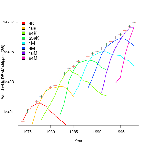
The plot below shows sales volume, in gigabytes, of various sized DRAM chips over time. The simple story of exponential growth in sales volume (plus signs) hides the more complicated story of the rise and fall of succeeding generations of memory chips (code+data):
The Red Queens had a simple task, keep buying the latest products. The activities of the companies supplying the specialist equipment needed to build a chip fabrication plant has to be coordinated, a role filled by the International Technology Roadmap for Semiconductors (ITRS). The annual ITRS reports contain detailed specifications of the expected performance of the subsystems involved in the fabrication process.
Moore’s law is now dead, in that transistor doubling now takes longer than two years. Would transistor doubling time have taken longer than two years, or slowed down earlier, if:
- the ecosystem had not been dominated by two symbiotic companies, or did network effects make it inevitable that there would be two symbiotic companies,
- the Internet had happened at a different time,
- if software applications had quickly reached a good enough state,
- if cloud computing had gone mainstream much earlier.
Where are the industrial strength R compilers?
Why don’t compiler projects for the R language make it into production use? The few that have been written have remained individual experimental products, e.g., RLLVMCompile.
Most popular languages attract many compiler implementations. I’m not saying that any of these implementations have more than a handful of users, that they implement the full language (a full implementation is not common), or that they fulfil any need other than their implementers desire to build something.
A commonly heard reason for the lack of production R compilers is that it is not worth the time and effort, because most of an R program’s time is spent in the library code which is written in a compiled language (e.g., C or Fortran). The fact that it is probably not worth the time and effort has not stopped people writing compilers for other languages, but then I think that the kind of people who use R tend not to be the kind of people who want to spend their time writing compilers. On the whole, they are the kind of people who are into statistics and data analysis.
Is it true that that most R programs spend most of their time executing library code? It’s certainly true for me. But I have noticed that a lot of the library functions executed by my code are written in R. Also, if somebody uses R for all their programming needs (it might be the only language they know), then their code might not be heavily library dependent.
I was surprised to read about Tierney’s byte code compiler, because his implementation is how I thought the R-core’s existing implementation worked (it does now). The internals of R is based on 1980s textbook functional techniques, and like many book implementations of the day, performance is dependent on the escape hatch of compiled code. R’s implementers wisely spent their time addressing user concerns, which revolved around statistics and visual presentation, i.e., not internal implementation technicalities.
Building an R compiler is easy, the much harder and time-consuming part is the runtime system.
Threaded code is a quick and simple approach to compiler implementation. R source gets mapped to a sequence of C function calls, with these functions proving a wrapper to library functions implementing the appropriate basic functionality, e.g., add two vectors. This approach has been the subject of at least one Master’s thesis. Thesis implementations rarely reach production use because those involved significantly underestimate the work that remains to be done, which is usually a lot more than the original implementation.
A simple threaded code approach provides a base for subsequent optimization, with the base having a similar performance to an interpreter. Optimizing requires figuring out details of the operations performed and replacing generic function calls with ones designed to be fast for specific cases, or even better replacing calls with inline code, e.g., adding short vectors of integers. There is a lot of existing work for scripting languages and a few PhD thesis researching R (e.g., Wang). The key technique is static analysis of R source.
Jan Vitek is running what appears to be the most active R compiler research group, at the moment e.g., the Ř project. Research can be good for uncovering language usage and trying out different techniques, but it is not intended to produce industry strength code. Lots of the fancy optimizations in early versions of the gcc C compiler started life as a PhD thesis, with the respective individual sometimes going on to spend a few years creating a production quality version for the released compiler.
The essential ingredient for building a production compiler is persistence. There are an awful lot of details that need to be sorted out (this is why research project code does not directly translate to production code, they ignore ‘minor’ details in order to concentrate on the ‘interesting’ research problem). Is there a small group of people currently beavering away on a production quality compiler for R? If there is, I can understand being discrete, on long-term projects it can be very annoying to have people regularly asking when the software is going to be released.
To have a life, once released, a production compiler needs to attract users, who are often loyal to their current compiler (because they know that their code works for this compiler); there needs to be a substantial benefit to entice people to switch. The benefit of compiling R to machine code, rather than interpreting, is performance. What performance improvement is needed to attract a viable community of users (there is always a tiny subset of users who will pay lots for even small performance improvements)?
My R code is rarely cpu bound, so I am not in the target audience, no matter what the speed-up. I don’t have any insight in the performance problems experienced by the R community, and have no idea whether a factor of two, five, ten or more would be enough.
Scientific management of software production
When Frederick Taylor investigated the performance of workers in various industries, at the start of the 1900’s, he found that workers organise their work to suit themselves; workers were capable of producing significantly more than they routinely produced. This was hardly news. What made Taylor’s work different was that having discovered the huge difference between actual worker output and what he calculated could be achieved in practice, he was able to change work practices to achieve close to what he had calculated to be possible. Changing work practices took several years, and the workers did everything they could to resist it (Taylor’s The principles of scientific management is an honest and revealing account of his struggles).
Significantly increasing worker output pushed company profits through the roof, and managers everywhere wanted a piece of the action; scientific management took off. Note: scientific management is not a science of work, it is a science of the management of other people’s work.
The scientific management approach has been successfully applied to production where most of the work can be reduced to purely manual activities (i.e., requiring little thinking by those who performed them). The essence of the approach is to break down tasks into the smallest number of component parts, to simplify these components so they can be performed by less skilled workers, and to rearrange tasks in a way that gives management control over the production process. Deskilling tasks increases the size of the pool of potential workers, decreasing labor costs and increasing the interchangeability of workers.
Given the almost universal use of this management technique, it is to be expected that managers will attempt to apply it to the production of software. The software factory was tried, but did not take-off. The use of chief programmer teams had its origins in the scarcity of skilled staff; the idea is that somebody who knows what they were doing divides up the work into chunks that can be implemented by less skilled staff. This approach is essentially the early stages of scientific management, but it did not gain traction (see “Programmers and Managers: The Routinization of Computer Programming in the United States” by Kraft).
The production of software is different in that once the first copy has been created, the cost of reproduction is virtually zero. The human effort invested in creating software systems is primarily cognitive. The division between management and workers is along the lines of what they think about, not between thinking and physical effort.
Software systems can be broken down into simpler components (assuming all the requirements are known), but can the implementation of these components be simplified such that they can be implemented by less skilled developers? The process of simplification is practical when designing a system for repetitive reproduction (e.g., making the same widget again and again), but the first implementation of anything is unlikely to be simple (and only one implementation is needed for software).
If it is not possible to break down the implementation such that most of the work is easy to do, can we at least hire the most productive developers?
How productive are different developers? Programmer productivity has been a hot topic since people started writing software, but almost no effective research has been done.
I have no idea how to measure programmer productivity, but I do have some ideas about how to measure their performance (a high performance programmer can have zero productivity by writing programs, faster than anybody else, that don’t do anything useful, from the client’s perspective).
When the same task is repeatedly performed by different people it is possible to obtain some measure of average/minimum/maximum individual performance.
Task performance improves with practice, and an individual’s initial task performance will depend on their prior experience. Measuring performance based on a single implementation of a task provides some indication of minimum performance. To obtain information on an individual’s maximum performance they need to be measured over multiple performances of the same task (and of course working in a team affects performance).
Should high performance programmers be paid more than low performance programmers (ignoring the issue of productivity)? I am in favour of doing this.
What about productivity payments, e.g., piece work?
This question is a minefield of issues. Manual workers have been repeatedly found to set informal quotas amongst themselves, i.e., setting a maximum on the amount they will produce during a shift (see “Money and Motivation: An Analysis of Incentives in Industry” by William Whyte). Thankfully, I don’t think I will be in a position to have to address this issue anytime soon (i.e., I don’t see a reliable measure of programmer productivity being discovered in the foreseeable future).
Performance variation in 2,386 ‘identical’ processors
Every microprocessor is different, random variations in the manufacturing process result in transistors, and the connections between them, being fabricated with more/less atoms. An atom here and there makes very little difference when components are built from millions, or even thousands, of atoms. The width of the connections between transistors in modern devices might only be a dozen or so atoms, and an atom here and there can have a noticeable impact.
How does an atom here and there affect performance? Don’t all processors, of the same product, clocked at the same frequency deliver the same performance?
Yes they do, an atom here or there does not cause a processor to execute more/less instructions at a given frequency. But an atom here and there changes the thermal characteristics of processors, i.e., causes them to heat up faster/slower. High performance processors will reduce their operating frequency, or voltage, to prevent self-destruction (by overheating).
Processors operating within the same maximum power budget (say 65 Watts) may execute more/less instructions per second because they have slowed themselves down.
Some years ago I spotted a great example of ‘identical’ processor performance variation, and the author of the example, Barry Rountree, kindly sent me the data. In the weeks before Christmas I finally got around to including the data in my evidence-based software engineering book. Unfortunately I could not figure out what was what in the data (relearning an important lesson: make sure to understand the data as soon as it arrives), thankfully Barry came to the rescue and spent some time doing software archeology to figure out the data.
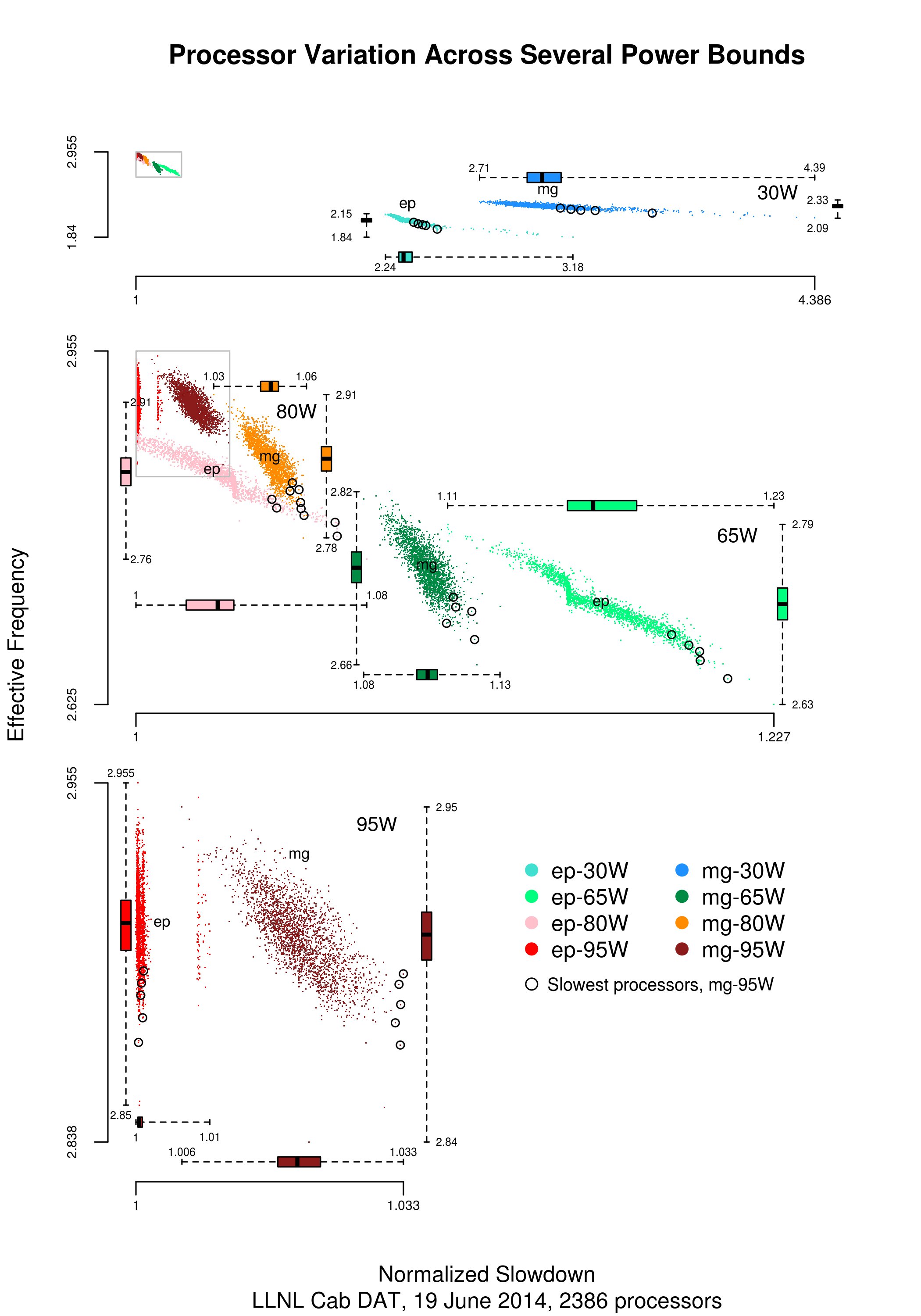
The original plots showed frequency/time data of 2,386 Intel Sandy Bridge XEON processors (in a high performance computer at the Lawrence Livermore National Laboratory) executing the EP benchmark (the data also includes measurements from the MG benchmark, part of the NAS Parallel benchmark) at various maximum power limits (see plot at end of post, which is normalised based on performance at 115 Watts). The plot below shows frequency/time for a maximum power of 65 Watts, along with violin plots showing the spread of processors running at a given frequency and taking a given number of seconds (my code, code+data on Barry’s github repo):

The expected frequency/time behavior is for processors to lie along a straight line running from top left to bottom right, which is roughly what happens here. I imagine (waving my software arms about) the variation in behavior comes from interactions with the other hardware devices each processor is connected to (e.g., memory, which presumably have their own temperature characteristics). Memory performance can have a big impact on benchmark performance. Some of the other maximum power limits, and benchmark, measurements have very different characteristics (see below).
More details and analysis in the paper: An empirical survey of performance and energy efficiency variation on Intel processors.
Intel’s Sandy Bridge is now around seven years old, and the number of atoms used to fabricate transistors and their connectors has shrunk and shrunk. An atom here and there is likely to produce even more variation in the performance of today’s processors.
A previous post discussed the impact of a variety of random variations on program performance.
Update start
A number of people have pointed out that I have not said anything about the impact of differences in heat dissipation (e.g., faster/slower warmer/cooler air-flow past processors).
There is some data from studies where multiple processors have been plugged, one at a time, into the same motherboard (i.e., low budget PhD research). The variation appears to be about the same as that seen here, but the sample sizes are more than two orders of magnitude smaller.
There has been some work looking at the impact of processor location (e.g., top/bottom of cabinet). No location effect was found, but this might be due to location effects not being consistent enough to show up in the stats.
Update end
Below is a png version of the original plot I saw:
Modular vs. monolithic programs: a big performance difference
For a long time now I have been telling people that no experiment has found a situation where the treatment (e.g., use of a technique or tool) produces a performance difference that is larger than the performance difference between the subjects.
The usual results are that differences between people is the source of the largest performance difference, successive runs are the next largest (i.e., people get better with practice), and the smallest performance difference occurs between using/not using the technique or tool.
This is rather disheartening news.
While rummaging through a pile of books I had not looked at in many years, I (re)discovered the paper “An empirical study of the effects of modularity on program modifiability” by Korson and Vaishnavi, in “Empirical Studies of Programmers” (the first one in the series). It’s based on Korson’s 1988 PhD thesis, with the same title.
There were four experiments, involving seven people from industry and nine students, each involving modifying a 900(ish)-line program in some way. There were two versions of each program, they differed in that one was written in a modular form, while the other was monolithic. Subjects were permuted between various combinations of program version/problem, but all problems were solved in the same order.
The performance data (time to complete the task) was published in the paper, so I fitted various regressions models to it (code+data). There is enough information in the data to separate out the effects of modular/monolithic, kind of problem and subject differences. Because all subjects solved problems in the same order, it is not possible to extract the impact of learning on performance.
The modular/monolithic performance difference was around twice as large as the difference between subjects (removing two very poorly performing subjects reduces the difference to 1.5). I’m going to have to change my slides.
Would the performance difference have been so large if all the subjects had been experienced developers? There is not a lot of well written modular code out there, and so experienced developers get lots of practice with spaghetti code. But, even if the performance difference is of the same order as the difference between developers, that is still a very worthwhile difference.
Now there are lots of ways to write a program in modular form, and we don’t know what kind of job Korson did in creating, or locating, his modular programs.
There are also lots of ways of writing a monolithic program, some of them might be easy to modify, others a tangled mess. Were these programs intentionally written as spaghetti code, or was some effort put into making them easy to modify?
The good news from the Korson study is that there appears to be a technique that delivers larger performance improvements than the difference between people (replication needed). We can quibble over how modular a modular program needs to be, and how spaghetti-like a monolithic program has to be.
Impact of group size and practice on manual performance
How performance varies with group size is an interesting question that is still an unresearched area of software engineering. The impact of learning is also an interesting question and there has been some software engineering research in this area.
I recently read a very interesting study involving both group size and learning, and Jaakko Peltokorpi kindly sent me a copy of the data.
That is the good news; the not so good news is that the experiment was not about software engineering, but the manual assembly of a contraption of the experimenters devising. Still, this experiment is an example of the impact of group size and learning (through repeating the task) on time to complete a task.
Subjects worked in groups of one to four people and repeated the task four times. Time taken to assemble a bespoke, floor standing rack with some odd-looking connections between components was measured (the image in the paper shows something that might function as a floor standing book-case, if shelves were added, apart from some component connections getting in the way).
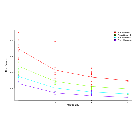
The following equation is a very good fit to the data (code+data). There is theory explaining why ") applies, but the division by group-size was found by suck-it-and-see (in another post I found that time spent planning increased with teams size).
applies, but the division by group-size was found by suck-it-and-see (in another post I found that time spent planning increased with teams size).
There is a strong repetition/group-size interaction. As the group size increases, repetition has less of an impact on improving performance.
![time = 0.16+ 0.53/{group size} - log(repetitions)*[0.1 + {0.22}/{group size}]](https://shape-of-code.com/wp-content/plugins/wpmathpub/phpmathpublisher/img/math_981.5_b0d171bba046801a68ce5dc8ae1d6115.png "time = 0.16+ 0.53/{group size} - log(repetitions)*[0.1 + {0.22}/{group size}]")
The following plot shows one way of looking at the data (larger groups take less time, but the difference declines with practice), lines are from the fitted regression model:
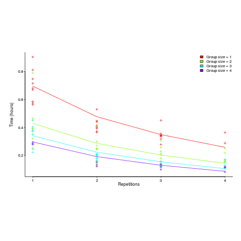
and here is another (a group of two is not twice as fast as a group of one; with practice smaller groups are converging on the performance of larger groups):
Would the same kind of equation fit the results from solving a software engineering task? Hopefully somebody will run an experiment to find out 🙂
Publishing information on project progress: will it impact delivery?
Numbers for delivery date and cost estimates, for a software project, depend on who you ask (the same is probably true for other kinds of projects). The people actually doing the work are likely to have the most accurate information, but their estimates can still be wildly optimistic. The managers of the people doing the work have to plan (i.e., make worst/best case estimates) and deal with people outside the team (i.e., sell the project to those paying for it); planning requires knowledge of where things are and where they need to be, while selling requires being flexible with numbers.
A few weeks ago I was at a hackathon organized by the people behind the Project Data and Analytics meetup. The organizers (Martin Paver & co.) had obtained some very interesting project related data sets. I worked on the Australian ICT dashboard data.
The Australian ICT dashboard data was courtesy of the Queensland state government, which has a publicly available dashboard listing digital project expenditure; the Victorian state government also has a dashboard listing ICT expenditure. James Smith has been collecting this data on a monthly basis.
What information might meaningfully be extracted from monthly estimates of project delivery dates and costs?
If you were running one of these projects, and had to provide monthly figures, what strategy would you use to select the numbers? Obviously keep quiet about internal changes for as long as possible (today’s reduction can be used to offset a later increase, or vice versa). If the client requests changes which impact date/cost, then obviously update the numbers immediately; the answer to the question about why the numbers changed is that, “we are responding to client requests” (i.e., we would otherwise still be on track to meet the original end-points).
What is the intended purpose of publishing this information? Is it simply a case of the public getting fed up with overruns, with publishing monthly numbers is seen as a solution?
What impact could monthly publication have? Will clients think twice before requesting an enhancement, fearing public push back? Will companies doing the work make more reliable estimates, or work harder?
Project delivery dates/costs change because new functionality/work-to-do is discovered, because the appropriate staff could not be hired and other assorted unknown knowns and unknowns.
Who is looking at this data (apart from half a dozen people at a hackathon on the other side of the world)?
Data on specific projects can only be interpreted in the context of that project. There is some interesting research to be done on the impact of public availability on client and vendor reporting behavior.
Will publication have an impact on performance? One way to get some idea is to run an A/B experiment. Some projects have their data made public, others don’t. Wait a few years, and compare project performance for the two publication regimes.
Time taken to compile a source file
How long will it take to compile a source file?
When computers were a lot slower than they are today, this question was of general interest. Job scheduling is more effective when reliable runtime estimates are available, and developers want to know if there is enough time to get a coffee before the compile finishes.
An embarrassing fact about compile time performance, used to be that a large percentage of compile time was spent doing lexical analysis [“The cost of lexical analysis”, I cannot find an online copy]. Why was this embarrassing? Compiler writers like to boast about all the fancy optimizations their compiler does; but doing fancy stuff consumes lots of resources, so why were compilers spending so much of their time doing simple things like lexical analysis? The reality was that fancy compiler optimizations were not commercially viable until developer computers contained tens of megabytes of memory, i.e., very few pre-1990 compilers did any real optimization (people are still fussing over lexer performance).
An analysis of the data in Captain Dennis Miller’s Masters thesis (late Rome period), finds compile time is proportional to the square root of the number of tokens in the source (code+data); more complicated models are a slightly better fit. Where did square root come from? I expected a linear relationship, but would be willing to go with log. The measurements are from Ada compilers in the mid 1980s. I know several people who worked on Ada compilers during that time, and they were implementing the latest fancy optimizations (Ada was going to be the next big thing and the venture capital was flowing; big companies, with big computers were going to be paying lots of money to use Ada, but then microcomputers came along). I think that square root is driven by OS resource limitations, the compilers are using lots of memory and a noticeable amount of time is spent swapping.
So computers got a lot faster and people lost interest in estimates of how long it would take to compile individual files. I have not seen any interest in predicting how long it would take to compile whole projects (just complaints about how long it takes). There has been some work on progress indicators, updated as compilation progresses, which is a step in the right direction. Perhaps somebody has recorded compile time information and thrown machine learning at it; I usually ignore machine learning papers applied to software engineering and perhaps I have missed something. Pointers to project compile time prediction work welcome.
Then along came just-in-time compilation. Now people want to estimate how long it will take to generate machine code from some intermediate form, that is being interpreted.
The plot below (thanks to Rafael Auler for kindly supplying the data from his paper) shows the time taken to generate code from functions containing a given number of LLVM instructions (an intermediate code), at optimization level O3. The red line is a regression fit to one of the ‘arms’ and shows constant time for less than 100’ish instructions and then a linear relationship. I have no idea why the time is roughly constant for a large number of functions.

There is a lot of variation for function containing the same number of instructions. This is to be expected when lots of different optimizations are being tried; sometimes a function will contain lots of the kind of code that a particular optimization spends lot of times process and sometimes the code will not contain anything interesting (i.e., no optimizations are found).
Main memory: the crucial component that vendors don’t mention
CPU performance hogs the limelight when people discuss the year-on-year increases in computing power that used to occur.
This focus on cpu performance was/is driven by marketing, the people with the money either don’t want customers thinking about the performance impact of main memory size or speed, or want them to treat the processor as the most important component of a computer. Vendors want processor performance to drive customer purchase decisions.
Hardware manufacturers used to entice new customers with low cost machines, containing minimal memory. Once a customer started to use their shiny new computer, they found that it did save them lots of time and money, but also they needed more memory (which could only be brought from the manufacturer and was not cheap).
The plot below shows the prices IBM charged for System 360s, in 1966. Anti-trust investigations uncover all kinds of interesting data, like selling low-spec equipment at a loss to entice customers and make life difficult for competitors (code+data for all plots).
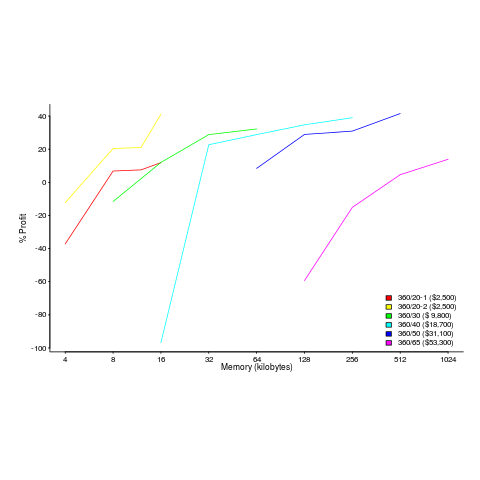
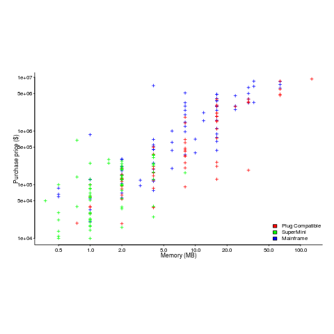
The plot below (data from the 19 Aug 1985 issue of ComputerWorld) shows how the price of computers increased as the minimum about of memory they supported increased.
Yes, in 1985 top end computers came with over 50M of memory; but most customers thought themselves lucky if they had a few megabytes.
If the processor is slow, it just takes longer for programs to run. If the computer does not have enough memory, programs cannot run. For most applications memory requirements are addressed first, followed by processor performance; memory requirements is the number one issue. The optimizations that commercial compilers could perform were limited by the memory capacity of developer machines.
Intel’s main line of business used to be selling memory chips, but these chips became commodity items as more companies entered the market; Intel bet the farm on selling processors and the rest is history. As a seller of a unique product it was/is in Intel’s interest to spend lots of money on marketing the benefits of processor performance; sellers of commodity items (such as memory chips) don’t have nearly as much to gain from generic product marketing, because customers may choose to buy from other sellers (in such markets sellers have to concentrate on marketing themselves).
Memory capacity/speed and cpu speed are two aspects of system performance; they need to be balanced to meet customer drive application requirements. The plot below shows the SPEC cpu integer performance of 4,332 systems running at various clock rates; the colors denote the different peak memory transfer rates of the memory chips in these systems (code+data).
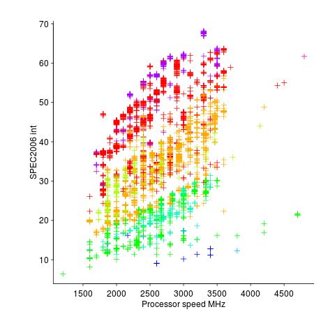
These days (and perhaps in the past, I don’t have any data), memory performance is a much better predictor of system performance, but vendors don’t have an incentive to market this fact.
Cost/performance analysis of 1944-1967 computers: Knight’s data
Changes In Computer Performance and Evolving Computer Performance 1963-1967, by Kenneth Knight, are the references to cite when discussing the performance of early computers. I suspect that very few people have read the two papers they are citing (citing without reading is a surprisingly common practice). Both papers were published in Datamation, a computer magazine whose technical contents could rival that of the ACM journals in the 1960s, but later becoming more of a trade magazine. Until the articles appeared on bitsavers.org they were only really available through national or major regional libraries.
Both papers contain lots of interesting performance and cost data on computers going back to the 1940s. However, I was not interested enough to type in all that data. This week I found high quality OCRed copies of the papers on the Internet Archive; my effort was reduced to fixing typos, which felt like less work.
So let’s try to reproduce Knight’s analysis of the data (code and data). Working in the mid-1960s, I imagine Knight did everything manually, with the help of mechanical calculators. I have the advantage of fancy software, a very fast computer and techniques that were invented after Knight did his analysis (e.g., generalized linear methods).
Each paper contains its own dataset: the first contains performance+cost data on 225 computers available between 1944 and 1963, while the second contains this information on 63 computers available between 1963 and 1967.
The dataset lists the computer name, the date it was introduced, number of operations per second and the number of seconds that can be rented for a dollar (most computer time used to be rented, then 25 years later personal computers came along and people got to own one, now, 25 years after that Cloud is causing a switch back to rental per second).
How are operations measured? The MIPS unit of measurement did not start to be generally used until the 1980s. Knight used 30 or so system characteristics, such as time to perform various arithmetic operations and I/O time, plus characteristics of scientific and commercial applications to calculate a value considered to be a representative scientific or commercial operation.
There is no mention of how seconds-per-dollar values were obtained. Did Knight ask customers or vendors? In a rental market, I imagine vendor pricing could be very flexible.
In the 1970s people started talking about Moore’s law, but in the 1960s there was Grosch’s law: Computer performance increases as the square of the cost, i.e., faster computers were cheaper to rent, for a given number of operations. Knight set out to empirically check Grosch’s law, i.e., he was looking for a quadratic fit.
Fitting a regression model to the 1950-1961 data, Knight obtained an exponent of 2.18, while I obtained 2.38 for commercial operations (using a slightly more sophisticated model, because I could); time on faster computers was cheaper than Grosch claimed. For scientific operations, Knight obtained 1.92, while I obtained 3.56; despite trying all sorts of jiggery-pokery I could not get a lower value. Unless Knight used very different values to the ones published in the ‘scientific’ columns, one of us has made a big mistake (please let me know if my code is wrong).
Fitting a regression model to the 1963-1967 data, I get figures (both around 2.85 and 2.94) that are roughly in agreement with Knight (2.5 and 3.1). Grosch’s law has broken down by 1963 (if it ever held for scientific operations).
The plot below shows operations per second against operationsseconds per dollar for the 1953-1961 data, with fitted lines for some specific years. It shows that while customers get fewer seconds per dollar on faster computers, the number of operations performed in those seconds is raised to the power of two+ (code and data):
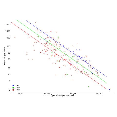
What other information can be extracted from the data? The 1953-1961 data shows seconds per dollar increased, over the whole performance range, by a factor of 1.15 per year, i.e., 15%, for both scientific and commercial; the 1963-1967 year-on-year increase jumps around a lot.
Recent Comments