The Shape of Code

Since it was created in the 1960s, the Norden-Rayleigh model of large project manpower has consistently outperformed, or close runner-up, other models in benchmarks (a large project is one requiring two or more man-years of effort). The accuracy of the Norden-Rayleigh model comes with a big limitation: a crucial input value to the calculation is the time at which project manpower peaks (which tends to be halfway through a project). The model just does not work for times before the point of maximum manpower.

Who is the customer for a model that predicts total project manpower from around the halfway point? Managers of acquisition contracts looking to evaluate contractor performance.

Not only does the Norden-Rayleigh model make predictions that have a good enough match with reality, there is some (slightly hand wavy) theory behind it. This post delves into Peter Norden’s derivation of the model, and some of the subsequent modifications. Norden work is the result of studies carried out at IBM Development Laboratories between 1956 and 1964, looking for improved methods of estimating and managing hardware development projects; his PhD thesis was published in 1964.

The 1950s/60s was a period of rapid growth, with many major military and civilian systems being built. Lots of models and techniques were created to help plan and organise these projects, two that have survived the test of time are the critical path method and PERT. As project experience and data accumulated, techniques evolved.

Norden’s 1958 paper “Curve Fitting for a Model of Applied Research and Development Scheduling” describes how a project consists of overlapping phases (e.g., feasibility study, deign, implementation, etc), each with their own manpower rates. The equation Norden fitted to cumulative manpower was: , where is project elapsed time, is total project manpower, and , , and are fitted constants. This is the logistic equation with added tunable parameters.

By the early 1960s, Norden had brought together various ideas to create the model he is known for today. For an overview, see his paper (starting on page 217): Project Life Cycle Modelling: Background and Application of the Life Cycle Curves.

The 1961 paper: “The decisions of engineering design” by David Marples was influential in getting people to think about project implementation as a tree-like collection of problems to be solved, with decisions made at the nodes.

The 1958 paper: The exponential distribution and its role in life testing by Benjamin Epstein provides the mathematical ideas used by Norden. The 1950s was the decade when the exponential distribution became established as the default distribution for hardware failure rates (the 1952 paper: An Analysis of Some Failure Data by D.J. Davis supplied the data).

Norden draws a parallel between a ‘shock’ occurring during the operation of a device that causes a failure to occur and a discovery of a new problem to be solved during the implementation of a task. Epstein’s exponential distribution analysis, along with time dependence of failure/new-problem, leads to the Weibull distribution. Available project manpower data consistently fitted a special case of the Weibull distribution, i.e., the Rayleigh distribution (see: Project Life Cycle Modelling: Background and Application of the Life Cycle Curves (starts on page 217).

The Norden-Rayleigh equation is: , where: is work completed, is total manpower over the lifespan of the project, , is time of maximum effort per unit time (i.e., the Norden/Rayleigh equation maximum value), and is project elapsed time.

Going back to the original general differential equation, before a particular solution is obtained, we have: , where is the amount of work left to do (it’s sometimes referred to as the learning curve). Norden assumed that: .

The 1980 paper: “An alternative to the Rayleigh curve model for software development effort” by F.N. Parr argues that the assumption of work remaining being linear in time is unrealistic, rather that because of the tree-like nature of problem discovery, the work still be to done, , is proportional to the work already done, i.e., , leading to: , where: is some fitted constant.

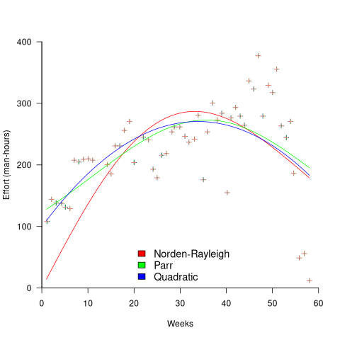
While the Norden-Rayleigh equation looks very different from the Parr equation, they both do a reasonable job of fitting manpower data. The following plot fits both equation to manpower data from a paper by Basili and Beane (code+data):

A variety of alternative forms for the quantity have been proposed. An unpublished paper by H.M. Hubey discusses various possibilities.

Some researchers have fitted a selection of equations to manpower data, searching for the one that gives the best fit. The Gamma distribution is sometimes found to provide a better fit to a dataset. The argument for the Gamma distribution is not based on any theory, but purely on the basis of being the best fitting distribution, of those tested.