Archive
Source code has a brief and lonely existence
The majority of source code has a short lifespan (i.e., a few years), and is only ever modified by one person (i.e., 60%).
Literate programming is all well and good for code written to appear in a book that the author hopes will be read for many years, but this is a tiny sliver of the source code ecosystem. The majority of code is never modified, once written, and does not hang around for very long; an investment is source code futures will make a loss unless the returns are spectacular.
What evidence do I have for these claims?
There is lots of evidence for the code having a short lifespan, and not so much for the number of people modifying it (and none for the number of people reading it).
The lifespan evidence is derived from data in my evidence-based software engineering book, and blog posts on software system lifespans, and survival times of Linux distributions. Lifespan in short because Packages are updated, and third-parties change/delete APIs (things may settle down in the future).
People who think source code has a long lifespan are suffering from survivorship bias, i.e., there are a small percentage of programs that are actively used for many years.
Around 60% of functions are only ever modified by one author; based on a study of the change history of functions in Evolution (114,485 changes to functions over 10 years), and Apache (14,072 changes over 12 years); a study investigating the number of people modifying files in Eclipse. Pointers to other studies that have welcome.
One consequence of the short life expectancy of source code is that, any investment made with the expectation of saving on future maintenance costs needs to return many multiples of the original investment. When many programs don’t live long enough to be maintained, those with a long lifespan have to pay the original investments made in all the source that quickly disappeared.
One benefit of short life expectancy is that most coding mistakes don’t live long enough to trigger a fault experience; the code containing the mistake is deleted or replaced before anybody notices the mistake.
Update: a few days later
I was remiss in not posting some plots for people to look at (code+data).
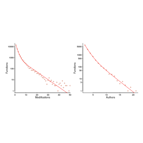
The plot below shows number of function, in Evolution, modified a given number of times (left), and functions modified by a given number of authors (right). The lines are a bi-exponential fit.
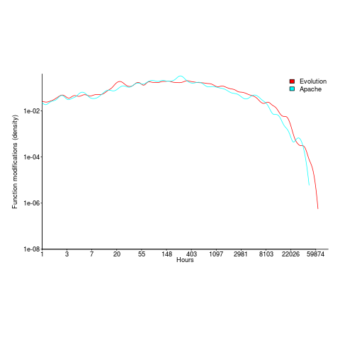
What is the interval (in hours) between between modifications of a function? The plot below has a logarithmic x-axis, and is sort-of flat over most of the range (you need to squint a bit). This is roughly saying that the probability of modification in hours 1-3 is the same as in hours 3-7, and hours, 7-15, etc (i.e., keep doubling the hour interval). At round 10,000 hours function modification probability drops like a stone.
Half-life of software as a service, services
How is software used to provide a service (e.g., the software behind gmail) different from software used to create a product (e.g., sold as something that can be installed)?
This post focuses on one aspect of the question, software lifetime.
The Killed by Google website lists Google services and products that are no more. Cody Ogden, the creator of the site, has open sourced the code of the website; there are product start/end dates!
After removing 20 hardware products from the list, we are left with 134 software services. Some of the software behind these services came from companies acquired by Google, so the software may have been used to provide a service pre-acquisition, i.e., some calculated lifetimes are underestimates.
The plot below shows the number of Google software services (blue) having a given lifetime (calculated as days between Google starting/withdrawing service), mainframe software from the 1990s (red; only available at yearly resolution), along with fitted exponential regression lines (code+data):
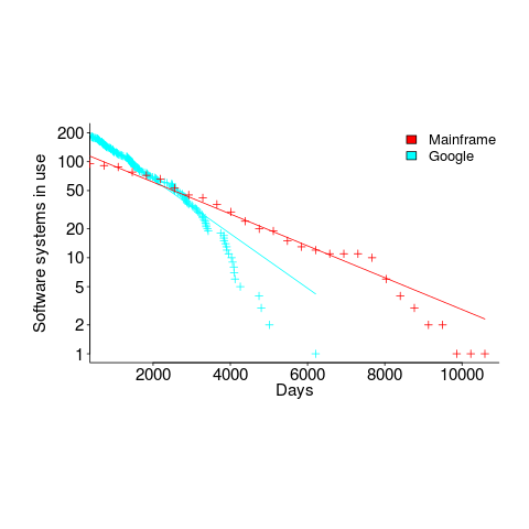
Overall, an exponential is a good fit (squinting to ignore the dozen red points), although product culling is not exponentially ruthless at short lifetimes (newly launched products are given a chance to prove themselves).
The Google service software half-life is 1,500 days, about 4.1 years (assuming the error/uncertainty is additive, if it is multiplicative {i.e., a percentage} the half-life is 1,300 days); the half-life of mainframe software is 2,600 days (with the same assumption about the kind of error/uncertainty).
One explanation of the difference is market maturity. Mainframe software has been evolving since the 1950s and probably turned over at the kind of rate we saw a few years ago with Internet services. By the 1990s things had settled down a bit in the mainframe world. Will software-based services on the Internet settle down faster than mainframe software? Who knows.
Based on this Google data, the cost/benefit ratio when deciding whether to invest in reducing future software maintenance costs, is going to have to be significantly better than the ratio calculated for mainframe software.
Software system lifetime data is extremely hard to find (this is only the second set I have found). Any pointers to other lifetime data very welcome, e.g., a collection of Microsoft product start/end dates 🙂
Break even ratios for development investment decisions
Developers are constantly being told that it is worth making the effort when writing code to make it maintainable (whatever that might be). Looking at this effort as an investment what kind of return has to be achieved to make it worthwhile?
Short answer: The percentage saving during maintenance has to be twice as great as the percentage investment during development to break even, higher ratio to do better.
The longer answer is below as another draft section from my book Empirical software engineering with R book. As always comments and pointers to more data welcome. R code and data here.
Break even ratios for development investment decisions
Upfront investments are often made during software development with the aim of achieving benefits later (e.g., reduced cost or time). Examples of such investments include spending time planning, designing or commenting the code. The following analysis calculates the benefit that must be achieved by an investment for that investment to break even.
While the analysis uses years as the unit of time it is not unit specific and with suitable scaling months, weeks, hours, etc can be used. Also the unit of development is taken to be a complete software system, but could equally well be a subsystem or even a function written by one person.
Let  be the original development cost and
  the yearly maintenance costs, we start by keeping things simple and assume is the same for every year of maintenance; the total cost of the system over
  years is:

If we make an investment of  % in reducing future maintenance costs with the expectations of achieving a benefit of
  %, the total cost becomes:
 + y*m*(1+i)*(1-b)")
and for the investment to break even the following inequality must hold:
 + y*m*(1+i)*(1-b) < d + y*m")
expanding and simplifying we get:

or:

If the inequality is true the ratio  is the primary contributor to the right-hand-side and must be greater than 1.
A significant problem with the above analysis is that it does not take into account a major cost factor; many systems are replaced after a surprisingly short period of time. What relationship does the ratio need to have when system survival rate is taken into account?
Let  be the percentage of systems that survive each year, total system cost is now:

where *(1-b)")
Summing the power series for the maximum of years that any system in a company’s software portfolio survives gives:
}/{1 - s}")
and the break even inequality becomes:
} < {b}/{i} + b")
The development/maintenance ratio is now based on the yearly cost multiplied by a factor that depends on the system survival rate, not the total maintenance cost
If we take >= 5 and a survival rate of less than 60% the inequality simplifies to very close to:

telling us that if the yearly maintenance cost is equal to the development cost (a situation more akin to continuous development than maintenance and seen in 5% of systems in the IBM dataset below) then savings need to be at least twice as great as the investment for that investment to break even. Taking the mean of the IBM dataset and assuming maintenance costs spread equally over the 5 years, a break even investment requires savings to be six times greater than the investment (for a 60% survival rate).
The plot below gives the minimum required saving/investment ratio that must be achieved for various system survival rates (black 0.9, red 0.8, blue 0.7 and green 0.6) and development/yearly maintenance cost ratios; the line bundles are for system lifetimes of 5.5, 6, 6.5, 7 and 7.5 years (ordered top to bottom)
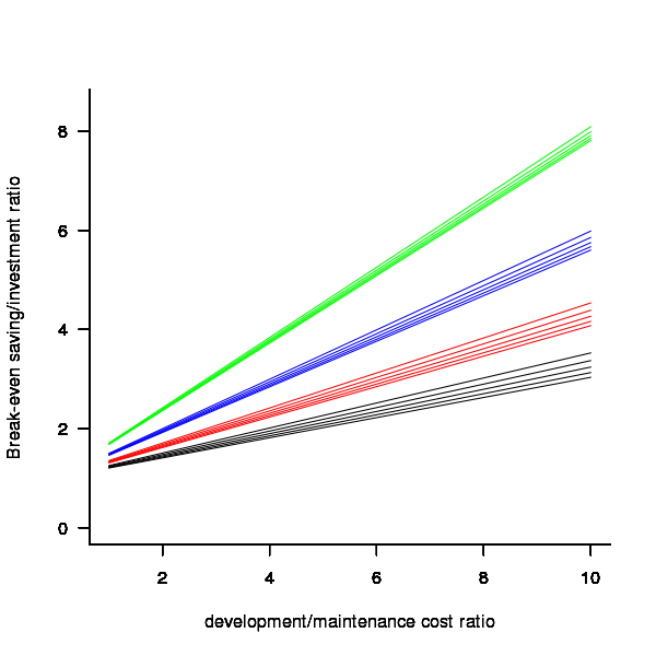
Figure 1. Break even saving/investment ratio for various system survival rates (black 0.9, red 0.8, blue 0.7 and green 0.6) and development/maintenance ratios; system lifetimes are 5.5, 6, 6.5, 7 and 7.5 years (ordered top to bottom)
Development and maintenance costs
Dunn’s PhD thesis <book Dunn_11> lists development and total maintenance costs (for the first five years) of 158 software systems from IBM. The systems varied in size from 34 to 44,070 man hours of development effort and from 21 to 78,121 man hours of maintenance.
The plot below shows the ratio of development to five year maintenance costs for the 158 software systems. The mean value is around one and if we assume equal spending during the maintenance period then  .
.
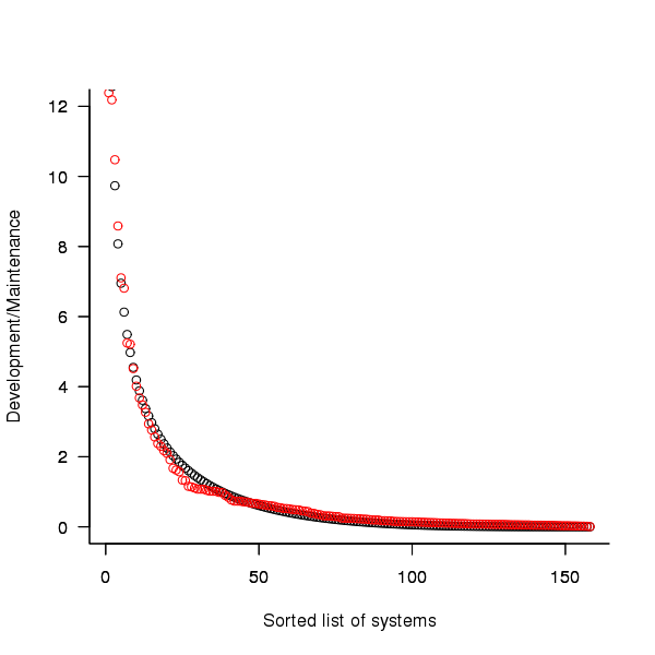
Figure 2. Ratio of development to five year maintenance costs for 158 IBM software systems sorted in size order. Data from Dunn <book Dunn_11>.
The best fitting common distribution for the maintenance/development ratio is the <Beta distribution>, a distribution often encountered in project planning.
Is there a correlation between development man hours and the maintenance/development ratio (e.g., do smaller systems tend to have a lower/higher ratio)? A Spearman rank correlation test between the maintenance/development ratio and development man hours gives:
|
showing very little connection between the two values.
Is the data believable?
While a single company dataset might be thought to be internally consistent in its measurement process, IBM is a very large company and it is possible that the measurement processes used were different.
The maintenance data applies to software systems that have not yet reached the end of their lifespan and is not broken down by year. Any estimate of total or yearly maintenance can only be based on assumptions or lifespan data from other studies.
System lifetime
A study by Tamai and Torimitsu <book Tamai_92> obtained data on the lifespan of 95 software systems. The plot below shows the number of systems surviving for at least a given number of years and a fit of an <Exponential distribution> to the data.
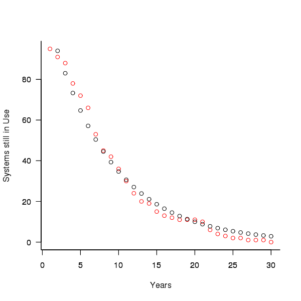
Figure 3. Number of software systems surviving to a given number of years (red) and an exponential fit (black, data from Tamai <book Tamai_92>).
The nls function gives  as the best fit, giving a half-life of 5.4 years (time for the number of systems to reduce by 50%), while rounding to
  gives a half-life of 6.6 years and reducing to
  a half life of 4.6 years.
It is worrying that such a small change to the estimated fit can have such a dramatic impact on estimated half-life, especially given the uncertainty in the applicability of the 20 year old data to today’s environment. However, the saving/investment ratio plot above shows that the final calculated value is not overly sensitive to number of years.
Is the data believable?
The data came from a questionnaire sent to the information systems division of corporations using mainframes in Japan during 1991.
It could be argued that things have stabilised over the last 20 years ago and complete software replacements are rare with most being updated over longer periods, or that growing customer demands is driving more frequent complete system replacement.
It could be argued that large companies have larger budgets than smaller companies and so have the ability to change more quickly, or that larger companies are intrinsically slower to change than smaller companies.
Given the age of the data and the application environment it came from a reasonably wide margin of uncertainty must be assigned to any usage patterns extracted.
Summary
Based on the available data an investment during development must recoup a benefit during maintenance that is at least twice as great in percentage terms to break even:
- systems with a yearly survival rate of less than 90% must have a benefit/investment rate greater than two if they are to break even,
- systems with a development/yearly maintenance rate of greater than 20% must have a benefit/investment rate greater than two if they are to break even.
The availanble software system replacement data is not reliable enough to suggest any more than that the estimated half-life might be between 4 and 8 years.
This analysis only considers systems that have been delivered and started to be used. Projects are cancelled before reaching this stage and including these in the analysis would increase the benefit/investment break even ratio.
Naming used to predict object lifetime
One of the most surprising empirical results I heard about this year was that the name of a Java object could (reasonably) reliably be used to predict its lifetime on the heap. Being a huge advocate of the importance of naming I should not have been surprised.
The author, Jeremy Singer, invited me to Manchester to talk about my own experiments and I heard about his group’s latest project investigating how to subdivide a Java program so that bits of it can be executed on different processors. I suggested various ways in which naming might be used to group semantically related functionality (would it do better than simple statement colocation you ask) and await to see if the group goes with any naming ideas (my suggestions were accompanied by a fair amount of arm waving, so I might have to wait a while).
Recent Comments