Archive
Early research on economies of scale for computer systems
Before microprocessor cost/performance wiped out (in the early 1990s) other cpu platforms (e.g., mainframes and minis), people argued that computer hardware benefited from economies of scale.
The claimed benefit was more bang for the buck, i.e., more compute for less money.
Checking this claim requires treating pre-microprocessor computer systems and the later microprocessor-based systems as two separate cases, because many of the factors driving costs and performance are very different.
Today’s large microprocessor-based computer systems achieve economies of scale through discounts from bulk purchases and spreading fixed costs across multiple systems. The data is available, and the economic analysis is straight forward.
A lack of reliable data on the costs of designing/building pre-microprocessor computer systems rules out an economic analysis of cost/performance from first principles. The data that was/is available is the cost of computer systems and some indicators of performance (such as instruction timings or benchmarks).
Now, the observed fact that the cost of compute was decreasing over time is unrelated to the claim that the cost of compute decreases as the size of the computer increases.
Assuming a power law relationship between computer cost,  , and size,
  , at a point in time, we have:
  , where
  is some constant. Economies of scale occur when:
In his detailed cost/performance analysis of computers between 1944-1967, Kenneth Knight treated computers launched in the same year as effectively occurring at the same time. He also built a single model, with year included as an explanatory variable, which means the fitted rate of decrease is the same over all years (rather than varying between years).
The plot below uses Knight’s 1953-1961 data, and shows operations per second against seconds per dollar (a confusing combination, but what Knight used), with fitted regression lines for three years using Knight’s model (code and data)
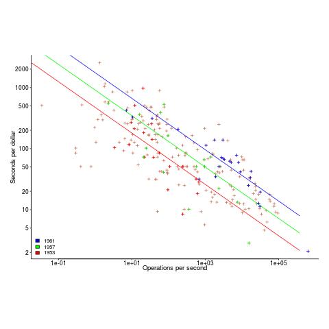
The fitted exponent for this form of x/y axis maps to a value which has , i.e., there are economies of scale.
It so happens that the value of the Knight’s fitted exponent is close to that proposed in a 1953 paper (“High speed arithmetic: The digital computer as a research tool”, no online copy):
It used to cost one cent to do a multiplication on a desk calculator; now it is more like four cents; but with these big machines we can do a million in an hour for $400, and that means twenty-five multiplications for a cent! I believe that there is a fundamental rule, which I modestly call Grosch's law, giving added economy only as the square root of the increase in speed-that is, to do a calculation ten times as cheaply you must do it one hundred times as fast. |
which did indeed become widely known as Grosch’s law.
Having been given a lucky kick-start by Knight (fitted individually, years are not close to Grosch’s law), checking for agreement with Grosch’s law became a focus for later studies. While various papers highlighted problems with the later data analysis (e.g., the regression techniques and sample noise producing mathematical artifacts), Grosch’s law ceased being a thing because mainframes/minicomputers ceased being a thing.
Did mainframe/mincomputers have economies of scale in the years after Knight’s data? It’s difficult to tell, the publicly available data is too sparse to support reliable analysis.
Cost/performance analysis of 1944-1967 computers: Knight’s data
Changes In Computer Performance and Evolving Computer Performance 1963-1967, by Kenneth Knight, are the references to cite when discussing the performance of early computers. I suspect that very few people have read the two papers they are citing (citing without reading is a surprisingly common practice). Both papers were published in Datamation, a computer magazine whose technical contents could rival that of the ACM journals in the 1960s, but later becoming more of a trade magazine. Until the articles appeared on bitsavers.org they were only really available through national or major regional libraries.
Both papers contain lots of interesting performance and cost data on computers going back to the 1940s. However, I was not interested enough to type in all that data. This week I found high quality OCRed copies of the papers on the Internet Archive; my effort was reduced to fixing typos, which felt like less work.
So let’s try to reproduce Knight’s analysis of the data (code and data). Working in the mid-1960s, I imagine Knight did everything manually, with the help of mechanical calculators. I have the advantage of fancy software, a very fast computer and techniques that were invented after Knight did his analysis (e.g., generalized linear methods).
Each paper contains its own dataset: the first contains performance+cost data on 225 computers available between 1944 and 1963, while the second contains this information on 63 computers available between 1963 and 1967.
The dataset lists the computer name, the date it was introduced, number of operations per second and the number of seconds that can be rented for a dollar (most computer time used to be rented, then 25 years later personal computers came along and people got to own one, now, 25 years after that Cloud is causing a switch back to rental per second).
How are operations measured? The MIPS unit of measurement did not start to be generally used until the 1980s. Knight used 30 or so system characteristics, such as time to perform various arithmetic operations and I/O time, plus characteristics of scientific and commercial applications to calculate a value considered to be a representative scientific or commercial operation.
There is no mention of how seconds-per-dollar values were obtained. Did Knight ask customers or vendors? In a rental market, I imagine vendor pricing could be very flexible.
In the 1970s people started talking about Moore’s law, but in the 1960s there was Grosch’s law: Computer performance increases as the square of the cost, i.e., faster computers were cheaper to rent, for a given number of operations. Knight set out to empirically check Grosch’s law, i.e., he was looking for a quadratic fit.
Fitting a regression model to the 1950-1961 data, Knight obtained an exponent of 2.18, while I obtained 2.38 for commercial operations (using a slightly more sophisticated model, because I could); time on faster computers was cheaper than Grosch claimed. For scientific operations, Knight obtained 1.92, while I obtained 3.56; despite trying all sorts of jiggery-pokery I could not get a lower value. Unless Knight used very different values to the ones published in the ‘scientific’ columns, one of us has made a big mistake (please let me know if my code is wrong).
Fitting a regression model to the 1963-1967 data, I get figures (both around 2.85 and 2.94) that are roughly in agreement with Knight (2.5 and 3.1). Grosch’s law has broken down by 1963 (if it ever held for scientific operations).
The plot below shows operations per second against operationsseconds per dollar for the 1953-1961 data, with fitted lines for some specific years. It shows that while customers get fewer seconds per dollar on faster computers, the number of operations performed in those seconds is raised to the power of two+ (code and data):
What other information can be extracted from the data? The 1953-1961 data shows seconds per dollar increased, over the whole performance range, by a factor of 1.15 per year, i.e., 15%, for both scientific and commercial; the 1963-1967 year-on-year increase jumps around a lot.
Recent Comments