The Shape of Code

The implementation of a project has a lifecycle that starts and finishes with zero people working on it. Between starting and finishing, the number of staff quickly grows to a peak before slowly declining. In a series of very hard to obtain papers during the early 1960s (chapter 5), Peter Norden created a large project staffing model described by the Rayleigh equation. This model was evangelized by Lawrence Putnam in the 1970s, who called it the Norden/Rayleigh model, while others sometimes now call it the Norden/Putnam, Putnam/Rayleigh, or some combination of names; Putnam’s papers can be hard to obtain.

The Norden/Rayleigh equation is:

where: is work completed, is total manpower over the lifespan of the project, , is time of maximum effort per unit time (i.e., the Norden/Rayleigh equation maximum value, which Putnam calls project development time), and is project elapsed time.

Norden’s model is only applicable to large projects (e.g., 2+ man-years), and Putnam points out that the staffing of small projects is usually a square wave, i.e., a number of staff are allocated at the start and this number remains the same until project completion.

As well as evangelizing Norden’s model, Putnam also created his own model; an equation connecting delivered lines of code, total manpower and project duration. The usually cited paper for this work is: “A General Empirical Solution to the Macro Software Sizing and Estimating Problem”, which can sometimes be found as a free download. I had always assumed that people did not take this model seriously, and it was not worth my time debunking it. The paper makes conjures hand-wavy connections between various equations which don’t seem to go anywhere, and eventually connects together a regression equation fitted to nine data points with an observation+assumption about another regression equation to create what Putnam calls the software equation: , where is delivered source code statements, and is a constant.

I recently read a 2014 paper by Han Suelmann debunking Putnam’s software equation, which led me to question my assumption about people not using Putnam’s model. Google Scholar shows 1,411 citations, with 133 since 2020. It looks like the software equation is still being taken seriously (or researchers are citing it because everybody else does; a common practice).

Why isn’t Putnam’s software equation worth treating seriously?

First, Putnam’s derivation of the software equation reads like a just-so story based on a tiny amount of data, and second a larger independent dataset does not show the pattern seen in Putnam’s data.

The derivation of the software equation starts by defining productivity as the number of delivered source code statements divided by the total manpower consumed to produce them, . Ok.

There is more certainty to a line fitted to a set of points that roughly follow a straight line, than to fit a line to points that follow a curve (because there are usually many ‘curve’ equations to choose from). The Norden/Rayleigh equation can be transformed to a form that is amenable to fitting a straight line, i.e., dividing by time and taking logs, as follows (which plugs in the value of ):

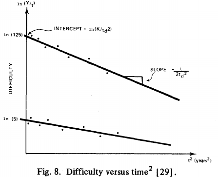
Putnam noticed (or perhaps it was the authors of the cited prepublication paper “Software budgeting model” by G. E. P. Box and L. Pallesen, which I cannot locate a copy of) that when plotting against : “If the number was small, it corresponded with easy systems; if the number was large, it corresponded with hard systems and appeared to fall in a range between these extremes.” Notice that in the screenshot of a figure from Putnam’s paper below, the y-axis is labelled “Difficulty”, not with the quantity actually plotted.

Based on an observation about easy/hard systems (it is never explained how easy/hard is measured) something called difficulty is defined to be: . No explanation is given for dropping the log scaling, or the possibility that some other relationship might hold.

The screenshot below is of a figure from Putnam’s paper, which plots the values of against for 13 projects. The fitted regression lines (the three lines are fitted using, 9, 2 and 2 points of the 13 projects) have the form , i.e., (I extracted the points and fitted ; code+extracted data):

With a bit of algebra, the two equations: and , can be combined to create the software equation.

Yes, Putnam’s software equation was hand-waved into existence by plucking a “difficulty” component from an observation about the behavior of projects in a regression model and equating it to a regression line fitted to nine points.

Are the patterns seen by Putnam found in other projects?

In the 1987 paper “Time-Sensitive Cost Models in the Commercial MIS Environment” D. Ross Jeffery used data from 47 projects to investigate the effort/time relationships used by Putnam to derive his software equation.

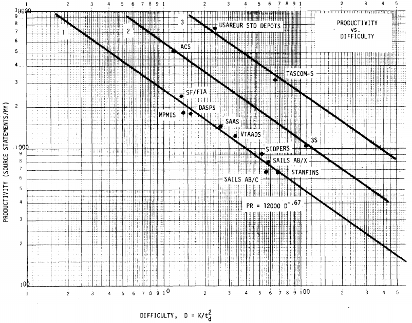
The plot below, of log(Difficulty) vs log(Productivity), shows what appears to be a random scattering of points, confirmed by failing to fit a regression model (code+extracted data):

No. The patterns seen by Putnam are not present in these projects. I don’t think that the difference in application domain is relevant (Putnam’s projects were for Military systems and Jeffery’s are for commercial projects). Norden’s model is not specific to software projects.

Jeffery’s uses a regression model to find: , the corresponding Putnam equation is: (the paper does not include the plot needed to extract the required data). The exponent might be claimed to be close enough, but the exponent is very different.

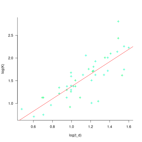
Jeffery’s paper includes a plot of against , and the plot below shows the extracted data (44 points), plus fitted regression line (code+extracted data):

The regression line has the form . This relationship further undermines assumptions made by Putnam, e.g., smaller systems are easier.

The Han Suelmann paper that triggered this post takes a very different approach to debunking Putnam’s model (he uses simulation to show that random data, drawn from a suitable distribution, can produce the patterns seen by Putnam).