Benchmarking string search algorithms
Searching a sequence of items for occurrences of a specific pattern is a common operation, and researchers are still discovering faster string search algorithms.
While skimming the paper Efficient Exact Online String Matching Through Linked Weak Factors by M. N. Palmer, S. Faro, and S. Scafiti, Tables 1, 2 and 3 jumped out at me. The authors put a lot of effort into benchmarking the performance of 21 search algorithms representing a selection of go-faster techniques (they wanted to show that their new algorithm, using hash chains, was the fastest; Grok explains the paper). I emailed the authors for the data, and Matt Palmer kindly added it to the HashChain Github repo. Matt was also generous with his time answering my questions.
The benchmark search involved three sequences of items, each of 100MB, a genome sequence, a protein sequence and English text. The following analysis if based on results from searching the English text. The search process returned the number of occurrences of the pattern in the character sequence.
The patterns to search for were randomly extracted from the sequence being searched. Eleven pattern lengths were used, ranging from 4 to 4,096 items in powers of 2 (the tables in the paper list lengths in the range 8 to 512). There were 500 runs for each length, with a different pattern used each time, i.e., a total of 5,500 patterns. Every search algorithm matched the same 5,500 patterns.
Some algorithms have tuneable parameters (e.g., the number of characters hashed), and 107 variants of the 21 algorithms were run, giving a total of 555,067 timing measurements (a 200ms time limit sometimes prevented a run completing).
To understand some of the patterns present in the timing results, it’s necessary to know something about how industrial strength string search algorithms work. The search pattern is first processed to create either a finite state machine or some other data structure. The matching process starts at the right of the pattern and moves left, comparing items. This approach makes it possible to skip over sequences of text that cannot match. For instance, if the current text character is X, this is fed into the finite state machine created from the pattern, and if X is not in the pattern, the matching process can move forward by the length of the pattern (if the pattern contains an X, the matching process skips forward the appropriate number of characters). This pattern shift technique was first implemented in the Boyer-Moore algorithm in 1977.
One consequence of skipping over sequences that cannot match, is that longer pattern enable longer skips, resulting in faster searches. The following plot shows the search time against pattern length for two algorithms; total time includes preprocessing the pattern and searching the text (red plus symbols have been offset by 10% to show both timings; code+data):
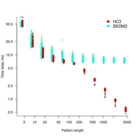
Why does the search time for HC3 (one variant of the author’s new algorithm) start to plateau and then start decreasing again? One possible cause of this saddle point is the cpu cache line width, which is 64 bytes on the system that ran the benchmarks. When the skip length is at least twice the cache line width, it is not necessary to read characters that would cause the filling of at least one cache line. As always, further research is needed.
What is the most informative method for comparing the algorithm/tool performance?
The most commonly used method is to compare mean performance times, and this is what the authors do for each pattern length. A related alternative, given that different patterns are used for each run, is to compare median times, on the basis that users are interested in the fastest algorithm across many patterns. When variance in the search times is taken into account, there is no clear winner across all pattern lengths (the uncertainty in the mean value is sometimes larger than the difference in performance).
Comparing performance across pattern lengths is interesting for algorithm designers, but users want a single performance value. The traditional approach to building a single model, that would include pattern length and algorithm, is to fit a regression model. However, this approach requires that the change in performance with pattern length roughly have the same form across all algorithms. The plot above clearly shows two algorithms with different forms of change of timing behavior with pattern length (other algorithms exhibit different behaviors).
A completely different modelling approach is to treat each pattern search as a competition between algorithms, with algorithms ranked by search time (fastest first). In this approach, the relative performance of each algorithm is ranked; there are 500 ranks for each pattern length. The fitted model can be used to calculate the probability, over all patterns, that algorithm A1 will be faster than algorithm A2.
Readers might be familiar with the Bradley-Terry model, where two items are ranked, e.g., the results from football games played between pairs of teams during a season. When more than two items are ranked, a Plackett-Luce model can be fitted. The output from fitting these models is a value,  , for each of the algorithms, e.g.,
  . The probability that algorithm
 A1 will rank higher than Algorithm A2 is calculated from the expression:
 , this expression can also be written as:
Switch A1 and A2 to calculate the opposite ranking.
The probability that algorithm A1 ranks higher than Algorithm A2 which in turn ranks higher than Algorithm A3 is calculated as follows (and so on for more algorithms):

For ease of comparison, only the 53 algorithms with 500 sets of timing data for all pattern lengths was fitted. The following plot shows the fitted values for each algorithm (blue/green lines are standard errors, and names containing HC are some variant of the authors’ hash chain technique; code+data):
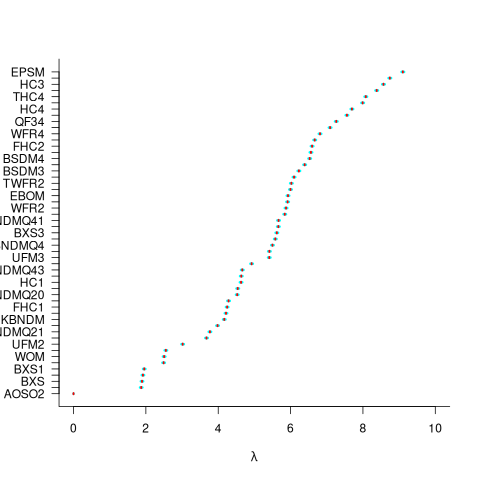
The EPSM algorithm makes use of the SSE and AVX instructions, supported by modern x86 processors, that can operate on up to 512 bits at a time.
The following table lists the fitted lambda values for the top eight ranked algorithm implementation:
 Algorithm    Lambda
      EPSM    9.103007
      THC3    8.743377
       HC3    8.567715
      FHC3    8.381220
      THC4    8.079716
      FHC4    7.991929
       HC4    7.695787
TWFR4 7.557796 |
The likelihood that EPSM will rank higher than THC3 is } right 0.59") .
.
This is better than random, and reflects the variability in algorithm performance, i.e., there is no clear winner.
It might be possible to extract more information from the data.
Some algorithms use of the same technique for part of their search process. Information on the techniques shared by algorithms can be added to the model as covariates. Assuming that a suitable fit is obtained, the model coefficients would indicate the relative impact of each technique on performance. I don’t know enough to select the techniques, and Matt is thinking about it.
Recent Comments